

Abstract
Congenital deafness affects developmental processes in the auditory cortex. In this study, local field potentials (LFPs) were mapped at the cortical surface with microelectrodes in response to cochlear implant stimulation. LFPs were compared between hearing controls and congenitally deaf cats (CDCs). Pulsatile electrical stimulation initially evoked cortical activity in the rostral parts of the primary auditory field (A1). This progressed both in the approximate dorsoventral direction (along the isofrequency stripe) and in the rostrocaudal direction. The dorsal branch of the wavefront split into a caudal branch (propagating in A1) and another smaller one propagating rostrally into the AAF (anterior auditory field). After the front reached the caudal border of A1, a “reflection wave” appeared, propagating back rostrally. In total, the waves took ∼13–15 ms to propagate along A1 and return back. In CDCs, the propagation pattern was significantly disturbed, with a more synchronous activation of distant cortical regions. The maps obtained from contralateral and ipsilateral stimulation overlapped in both groups of animals. Although controls showed differences in the latency–amplitude patterns, cortical waves evoked by contralateral and ipsilateral stimulation were more similar in CDCs. Additionally, in controls, LFPs with contralateral and ipsilateral stimulation were more similar in caudal A1 than in rostral A1. This dichotomy was lost in deaf animals. In conclusion, propagating cortical waves are specific for the contralateral ear, they are affected by auditory deprivation, and the specificity of the cortex for stimulation of the contralateral ear is reduced by deprivation.
Introduction
The sensory cortex represents features of physical stimuli topologically as well as temporally (in temporal firing patterns). Most investigations of cortical feature sensitivity so far have focused on only one type of representation. However, because of the parallel existence of both representations, coordinated spatiotemporal patterns of cortical activation are likely to occur. In spontaneous activity, spatiotemporal patterns of cortical activity have been described both under anesthesia and during sleep (Arieli et al., 1996; Destexhe et al., 1999). Because of technical reasons, only few studies concentrated on the spatiotemporal patterns of evoked activity. These studies described cortical waves evoked by visual stimuli using optical imaging (Arieli et al., 1996; Sharon and Grinvald, 2002; Benucci et al., 2007). Propagating waves emerge when neighboring groups of neurons depolarize and hyperpolarize with small delays; in this case, the activity “travels” through the cortex.
Propagating waves have also been demonstrated in the auditory cortex (Harrison et al., 1998; Nelken et al., 2004; Song et al., 2006). They are of cortical (or thalamocortical) origin, because they can be evoked also by intracortical microstimulation (Song et al., 2006). However, intrinsic optical imaging registers spatially smeared activity with low temporal resolution (Hess and Scheich, 1996; Spitzer et al., 2001; Nelken et al., 2004), catching only very slow propagating waves. Neurons, however, process signals within milliseconds. Only voltage-sensitive dyes could reveal waves within 100 ms poststimulus (Song et al., 2006). Activity has been restricted to isofrequency stripes in these studies, because sinusoidal acoustic stimulation has been used to demonstrate tonotopic organization with optical means (Harel et al., 2000; Versnel et al., 2002; Ojima et al., 2005; Song et al., 2006). Both thalamocortical and corticocortical interactions spread preferentially within isofrequency stripes (McMullen and de Venecia, 1993), but also over a significant distance orthogonal to them (McMullen and de Venecia, 1993; Velenovsky et al., 2003; Lee and Winer, 2008a). Thus, both the demonstrated slow velocity of auditory cortical waves and the observed limitation to the isofrequency stripe could result from methodological factors.
Most importantly, the functional significance of cortical propagating waves remains unclear. Demonstrating an effect of auditory experience on propagating waves would support their role in neuronal processing. This has not yet been attempted. The specificity of cortical waves with respect to the stimulated ear (contralaterality) would additionally emphasize their functional specificity and significance.
The present study investigates the effect of the complete absence of auditory experience on cortical propagating waves using electrophysiological methods. As a model of total auditory deprivation, congenitally deaf cats (CDCs) were used. These animals have no hearing experience at all (Heid et al., 1998). In this study, we demonstrate that a fast cortical wave evoked by cochlear implant stimulation propagates both within the isofrequency stripe and orthogonally to it, and that the wave is modified by the absence of hearing experience. Furthermore, we demonstrate that the wave characteristics also depend on the stimulated ear and that the contralaterality present in normal controls is reduced in the absence of hearing experience.
Materials and Methods
The present study was performed using eight animals: four CDCs and four hearing controls (HCs), all of adult age (>12 months). All the experiments were approved by the local state authority and were performed in compliance with the guidelines of the European Community for the Care and Use of Laboratory Animals (EU VD 86/609/EEC). The CDCs were selected from a colony of deaf white cats through early hearing screening using brainstem evoked responses with stimulation >120 dB sound pressure level (SPL) (Heid et al. 1998). The CDC has the unique advantage of an excellent preservation of spiral ganglion cells (Heid et al. 1998), so that the response to electrical stimulation is not affected by the extensive reductions of spiral ganglion cells described in deafened animals (Leake et al., 1999; Dodson and Mohuiddin, 2000). To prevent electrophonic hearing (electrical stimulation of hair cells) in hearing controls, these animals were deafened at the beginning of the experiment by intrascalar application of neomycin (Hartmann et al., 1984). Success of the deafening procedure was confirmed by the absence of brainstem evoked responses up to 120 dB SPL. In what follows, these adult, previously hearing, at the beginning of the acute experiment “hair cells-destroyed,” animals will be referred to as “hearing controls.” The adjective “hearing” does not refer to the functional state of the cochlea, but rather to the developmental and functional state of the central auditory system.
Cochlear implant.
The cochlear implant (CI) consisted of a medical-grade silicone carrier with six electrical contacts. There were five intrascalar contacts: a small golden ball at the tip (diameter, 0.8 mm) and four golden rings, with a distance of 1 mm between the electrodes (Behrendt, 1999). The gold contacts were connected to a seven-strand Teflon-coated stainless-steel braided wire. The intrascalar part of the implant was tapered in the apical direction from a diameter of 1.6 to 0.8 mm. The extracochlear silicone carrier had a diameter of 1.6 mm. An indifferent electrode was placed extracochlearly in the midline of the neck. The stimulation was with the apical most intracochlear electrode versus the neck electrode. The impedance of each implant electrode at 150 Hz stimulation was <5 kΩ.
Animal preparation.
The animals were premedicated with 0.25 mg of atropine intraperitoneally and initially anesthetized with ketamine hydrochloride (Ketavet; Parker Davis; 24.5 mg/kg) and propionylpromazine phosphate (Combelen; Bayer; 2.1 mg/kg). They were tracheotomized and artificially respirated with 50% O2 and 50% N2O, with the addition of 0.2–1.5% concentration isoflurane (Lilly) to maintain a controlled depth of anesthesia (Kral et al., 1999). End-tidal CO2 was monitored and kept <4%, and the core temperature was kept between 37.5 and 38.5°C using a homeothermic blanket. The status of the animal was further controlled by measurements of blood gas concentration, pH, bicarbonate concentration and base excess, glycemia, and oxygen saturation. A modified Ringer's solution containing bicarbonate and plasma expander was infused intravenously with additional bicarbonate depending on the status of the acidobasis. Monitoring and correction of acidobasis was performed every 12 h. The animals were maintained in the normal range of internal milieu parameters throughout the experiment.
The head of the animal was fixed in a stereotactic holder (Horsley-Clarke). Both bullae and ear canals were exposed. To record evoked auditory brainstem responses, a small trephination was drilled at the vertex and a silver ball electrode (diameter, 1 mm) was attached epidurally. The indifferent electrode used for the recordings was inserted medially in the neck muscles.
Deafness was verified at the beginning of the experiment using brainstem responses evoked with condensation clicks (50 μs duration; 200 stimulus repetitions; 33 stimuli per second) applied through a modified DT 48 speaker (Bayer Dynamics) at intensities >120 dB SPL. The membrane of the speaker was mounted at a distance of 2 cm from the tympanic membrane; sound was applied in a closed system into the external auditory meatus using a cone after the pinna was removed. The absence of acoustically evoked brainstem responses (including component I, generated within the auditory nerve) verified complete deafness. The same procedure was applied to determine the hearing status in controls (HCs). The hearing threshold determined with brainstem evoked responses was <40 dB SPL peak equivalent in all HCs used in the experiment. To prevent electrophonic responses, the hair cells in HCs were then destroyed by a slow instillation of 300 μl of neomycin sulfate into the scala tympani (within 5 min). The neomycin was left in place for additional 5 min followed by a slow instillation of Ringer's solution to wash out the neomycin. Absence of brainstem evoked responses verified a successful deafening procedure.
Electrical stimulation.
For electrical stimulation, cochlear implants were inserted bilaterally into the cochlea through the round window. Care was taken to ensure comparable insertion depth bilaterally: in each ear, the criterion was that the basal-most electrode of the implant was just recognizable behind the rim of the round window. During the electrophysiological experiment, charge-balanced pulses (200 μs/phase; repetition rate, 2 Hz; 100 stimuli) were applied to the cochlear implant in monopolar configuration. Stimulation was performed with optically isolated current sources (CS1; Otoconsult). To verify comparable positions of both cochlear implants, electrically evoked brainstem responses with single biphasic pulses were recorded and the lowest current levels evoking a brainstem response were determined. If the thresholds for stimulation of the left and the right ear differed by >2 dB, the ear with higher thresholds was reimplanted and the thresholds were remeasured. Similar threshold and similar insertion depth secured a comparable excitation spread in both auditory nerves.
Determination of cortical threshold currents.
A craniotomy was performed above the auditory cortex and the dura was removed. The cortex was photographed to document the recording positions. To find the stimulation intensity for subsequent mapping, the lowest current levels evoking a cortical response (threshold levels) were determined. Using an x–y–z micromanipulator enabling movements in all three directions with a precision of 1 μm, a silver-ball macroelectrode (diameter, 1 mm) was positioned on the surface and cortical thresholds at nine cortical positions covering the primary auditory cortex (field A1) were determined to find the value of the lowest cortical threshold. The dorsal end of the posterior ectosylvian sulcus was used as a reference point. Signals were preamplified (60 dB by Otoconsult V2 Low-Impedance Amplifier), amplified at a second stage (20 dB by Otoconsult Amplifier-Filter F1; filters, 0.010–10 kHz) and averaged (100 sweeps; repetition rate, 1.57 Hz). The resulting local field potentials (LFPs) were recorded using custom-made software programmed by the principal author using a 16-bit National Instruments MIO Card. The signals were stored and threshold current levels were evaluated at all recording positions with a precision of ±1 dB. These recordings determined the minimal stimulation current required for contralateral stimulation (CoS) and ispilateral stimulation (IpS) to evoke a cortical response at one or more of the recording positions (“cortical threshold current”).
Cortical mapping.
Cortical mapping was performed using a Ringer-filled glass microelectrode (impedance, ∼4 MΩ). Field potentials on the cortical surface were recorded at 100–150 cortical positions during stimulation with the cochlear implant using biphasic pulses (200 μs/phase; stimulation at the ipsilateral and also contralateral ear; stimulation current 10 dB above the lowest cortical threshold determined with the macroelectrode). To obtain the evoked LFP, recordings were averaged over 100 stimulus presentations (repetition rate, 2 Hz). Only averaged LFPs were evaluated in the present study. Consequently, the ongoing background activity could not be quantified from these data. With regard to the morphology of LFPs, the following terminology was used: Positive components were labeled “P,” and negative, “N,” with indexing increasing with time. Responses with latencies <100 ms were considered middle-latency responses and were signified by index letters “a” to “c.” Only the largest component (Pa) was used for component-specific analysis of amplitude–latency correlations and aural specificity in the present study.
Cortical activity was evaluated in terms of activation maps, with each map reflecting the amplitudes of the LFPs at all recording positions at the given poststimulus time, with linear interpolation of the activity between the recording positions (spatial interpolation). These cortical activation maps were constructed from the microelectrode recordings using custom-made software written in MatLab (Mathworks). Spatiotemporal activity patterns were obtained by presenting these maps sequentially in steps of 1 ms. To study the temporal features of the responses independently of amplitude variations, the LFPs were additionally amplitude-normalized by their maximum positive amplitude. The such-obtained normalized LFPs (nLFPs) were used to study propagation waves only. Orientation on the cortical surface was based on the sulcal pattern (Reale and Imig, 1980; Lee and Winer, 2008a,b).
Center of gravity.
To quantify the movement of the activity patterns, a function analogous to the center of gravity (COG) was computed at each time t, replacing the weight at each coordinate [x,y] by the amplitude of the nLFP at the corresponding location as follows:
 Here, nLFP(t)j represents the amplitude-normalized field potential recorded at position j at time t, and xj and yj are the coordinates of the jth recording position. As the focus of this analysis was in revealing the temporal spread of activity in the cortex, only amplitude-normalized LFPs were used for computation of COG. From these data, the velocity of the COG could be determined. For this calculation, the summed distance traveled by the center of gravity was computed within a moving window of 5 ms and given in micrometers per millisecond. During the first 6 ms, the calculated position of the COG was driven by spontaneous activity (was “random”) and then “jumped” onto an initial position near the center of A1. This abrupt change, although triggered by the first influence of the stimulus on the cortex, caused an erroneous peak in the propagation velocity. Therefore, the velocity of COG in the first 6 ms was blanked.
Contralateral and ipsilateral stimulation.
To compare the propagation waves for contralateral and ipsilateral stimulation (CoS and IpS), the Euclidean distance of the center of gravity for CoS and IpS was computed for each millisecond. These distances were subsequently compared between CDCs and HCs.
Additionally, from the positive amplitudes of LFPs for contralateral and ipsilateral stimulation at time t, a contralaterality index was computed for each recording site j using the following formula:
 where LFPc(t)j represents the amplitude of the LFP evoked by the CoS at the recording position j and time t, and LFPi(t)j represents the corresponding LFP evoked by ipsilateral stimulation. This index was computed for all positions at every millisecond poststimulus. If both LFPs were <50 μV, the contralaterality index was set to 0 to avoid random fluctuations of the LFPs affecting the map. Similarly, ipsilaterality indices were computed to better visualize the positions showing similar responses to both kind of stimulation in contrast to nonresponsive sites.
To quantify the difference in morphology of the LFPs evoked by contralateral and ipsilateral stimulation for each recording position j, the dissimilarity index (D) was used as follows (Massey and Denton, 1993):
 where LFPc represents the LFP evoked by the contralateral stimulation, and LFPi represents the LFP evoked by ipsilateral stimulation. At each sampled time (T), the amplitude of the LFP was divided by its temporal integral over the 100 ms after stimulus, and the summed difference of these for contralateral and ipsilateral stimulation was taken as a measure of dissimilarity. The dissimilarity index is not dependent on the maximum amplitude of the signal, because it is normalized to the temporal integral. If the two LFPs were the same with opposite polarity, D would reach 1, whereas if they were identical signals, it would be 0.
For statistical comparisons, the following procedures were used (Sachs, 1968): Data that showed a normal distribution (Pearson–Stephens's test, 10% significance level) (Sachs, 1968) were tested using two-tailed t test (5% significance level). For those data that were not normally distributed, a two-tailed Wilcoxon–Mann–Whitney's test was used (5% significance level). Testing was performed using Systat 11 (Systat Software) and the Statistics Toolbox from MatLab (Mathworks).
Results
This study recorded LFPs at the cortical surface in response to electrical stimulation of the auditory nerve. The initial orientation at the cortical surface was based on anatomical landmarks (the sulcal pattern) (Fig. 1A).

Functional organization of the primary auditory cortex of hearing controls with contralateral electrical stimulation (monopolar configuration). A, Image of the exposed cortex of the right hemisphere in one of the HCs with the designation of cortical areas based on anatomical landmarks. AAF, Anterior auditory field; A1, primary auditory field; ED, dorsal part of the posterior ectosylvian gyrus; PAF, posterior auditory field; A2, secondary auditory field; AEF, anterior ectosylvian field; SSS, superior sylvian sulcus; PES, posterior ectosylvian sulcus; AES, anterior ectosylvian sulcus. Below, Color-coded functional map of responses at 12 ms after stimulus with overlaid numbered recording positions. The crosses on the photograph and the activation map are used for alignment purposes. The dashed black line represents the central narrow line. B, Examples of LFPs at different recording positions with the cortical location indicated in the respective title. Similar morphology of LFPs sampled at different times demonstrates the reproducibility of the method. Also, characteristic differences at different positions are discernible. Sample positions in the map (A) are marked by the symbols shown in the corner of each panel. C, The 100 μV contours of the individual hot spots from all four hearing controls (individual animals shown in different color). As reference structures, the AES, PES, and the position and orientation of the central narrow line was used. The blue dashed line represents the overlapping central narrow line after alignment of the maps from each animal.
LFP morphology and reproducibility
Recordings were performed by moving one microelectrode along the primary auditory cortex. Although only the invariant portion of the cortical response, the evoked LFP, was evaluated at each position, the time difference between different recordings could have affected the recorded signals. As a test of reproducibility, LFPs recorded from adjoining positions taken at different times were compared. Even if taken more than an hour later, the LFPs still showed very similar morphology (Figs. 1, 5) (each position required >1 min for a recording; thus, the number of the position also approximately indicates the amount of time that has passed since the beginning of the recording session). The waveform comparisons in these figures illustrate that the morphology of LFPs was much more dependent on position than on the time the recording was taken.
The spatial resolution of this technique was high: if transitions in the morphology of LFPs with cortical position took place, they were discernible as abrupt changes even at positions separated only by few hundred micrometers (Fig. 1). The mapping method is simple and allows the analysis of phenomena that so far could only be addressed using optical imaging techniques.
The morphology of the recorded field potentials was consistent with previous studies (cf. Kral et al., 2002). The first components of evoked responses were observed in the latency range of 8–20 ms, most frequently between 9 and 12 ms. In some regions of A1, a positive component dominated in this latency range (designated as Pa) (Fig. 1B), generating “hot spots” in the cortical map (Fig. 1A, bottom). In other regions of A1 in HCs, the Pa component was smaller or not observed at all and activity was dominated by a negative component (Nb) (Fig. 1B, “A1: Negative spot”).
Hearing controls
Spatial distribution of electrically evoked responses
When cortical activity was evaluated in terms of the maximum amplitude of LFPs, consistent with previous studies two to three cortical hot spots were observed (Fig. 1A, bottom). The value of the maximum amplitude varied between individual animals (see below). At least two of the hot spots were clearly located within the primary auditory cortex as defined by anatomical landmarks [i.e., between superior sylvian sulcus (SSS), posterior ectosylvian sulcus (PES), and anterior ectosylvian sulcus (AES)] (Fig. 1A, top). The hot spots were designated in the following way: HS1 was the most rostrodorsal spot, HS2 the rostroventral one, and HS3 the caudalmost hot spot. HS2 in some animals appeared near the dorsal end of AES, in part invading into the AES, sometimes even extending rostrally from it (Fig. 1A). Therefore, HS2 might include nonprimary areas ventral from anterior auditory field (AAF). However, because of the small latency, as found in HS1 and HS3, we assume that HS2 includes mainly A1 and possibly AAF. In some animals, a participation of nonprimary auditory areas in the rostral section of this hot spot is possible.
As a rule, HS1 was located dorsally and caudally from the dorsal end of AES. This corresponded to the position of the field A1, extending to the border between A1 and AAF (Phillips and Irvine, 1982; Schreiner and Urbas, 1986; Lee and Winer, 2008b). HS3 was located more caudally within A1 (corresponding to the low-frequency region of A1). This spot was characterized by a smaller amplitude and a similar latency to HS1 and HS2.
The LFPs recorded at different sites of the mapped cortex had a region-specific morphology (Fig. 1B). Within the primary areas, responses had a high amplitude and one or two positive components (Pa and Pb), generating the hot spots. Between HS1 and HS3 was a prominent negative region characterized by the near absence of positive components and the presence of an Nb component (Fig. 1B, “A1: Negative spot”). The narrow region separating HS1 from HS2 (central narrow line) was characterized by a short-duration small amplitude Pa, followed by a sharp and shallow Nb, further followed by a longer-duration Pb component (Fig. 1B, “HS1–HS2”). This line extended further caudally in the direction of HS3. It could be observed in all hearing controls and was used as a landmark for mapping.
Most rostral parts of HS1, most likely located already within AAF (based on anatomical landmarks), showed a high-amplitude sharp Pa component closely followed by sharp Nb and Pb components (Fig. 1B, “A1–AAF”).
Border positions at the caudal and ventral part of A1 were characterized by longer latency, smaller amplitude, and longer duration Pa components (Fig. 1B, “A1–A2”). These regions most likely correspond to nonprimary auditory fields, the dorsal part of the posterior ectosylvian gyrus (ED), posterior auditory field (PAF), and secondary auditory field (A2). Dorsally, the belt region in the cat (field DZ) (Lee and Winer, 2008a,b) is partially hidden in the depths of the SSS, with ventral boundaries functionally not clearly specified. The maps obtained from this study possibly included activity also from this field, although the LFPs were not obviously different from those from field A1.
Using these LFP characteristics, hot spots and the central narrow line were identified in all animals. To compare the reproducibility of the organization of hot spots, the 100 μV contour of each hot spot was constructed for every animal. The individual contour maps were then slightly resized so that the position of the posterior and the anterior ectosylvian sulcus overlapped in all animals. In addition, the contour maps were aligned with regard to the central narrow line (Fig. 1C). Despite a certain variability in the extent and shape of the hot spots, their position overlapped well in all HCs (Fig. 1C), HS3 having a slightly higher variability in position. HS2 was not observed in one hearing control. In general, however, the cortical activation maps were clearly reproducible between animals.
Dynamics of spatiotemporal waves
Using the computation of cortical activation maps, the spatiotemporal dynamics of evoked responses can be revealed with a millisecond resolution. The dynamics of this data set were partly obscured by large responses that dominated the map. Obviously, each stimulus has some cortical representation and will evoke a more or less structured amplitude map in field A1. However, because of intrinsic horizontal connections in the auditory cortex and intraareal spread of activity via thalamocortical projections (Velenovsky et al., 2003; Lee and Winer, 2008a), activity can recruit larger cortical regions, although with smaller absolute amplitudes. To study the temporal features of the responses independently of amplitude variations, the LFPs were amplitude normalized by their maximum positive amplitude to obtain nLFPs. After this procedure, at each position the maximum positive amplitude of the nLFP was unitary. Through the use of such an approach, distinct progression waves became evident (Fig. 2). In all investigated HCs, the “initiating spot” was located at or near the rostral portion of the central narrow line. The first response was prominent at a latency of 7–8 ms. An initial wave progressed from the central narrow line dorsally and ventrally (into HS1 and HS2) (Fig. 2). It reached the dorsal and ventral extent of A1 within 3–6 ms. The dorsal branch was split into two wavefronts, one progressing rostrally (into AAF) and one progressing caudally (into A1) (Fig. 3). The caudal part swept across the field A1 and approached field ED. In some animals, this caudal wave was split into two branches, a ventral one and a dorsal one, that fused at the caudal end of A1. Afterward, the activation front returned from the border of field ED rostrally, heading toward the negativity zone within the next few milliseconds (reflection wave). In the microdynamics, some interindividual variability could be observed (Fig. 2) (for movies, see supplemental material, available at www.jneurosci.org). This is not surprising, because the tonotopic arrangement of the cortex also shows substantial interindividual variability (Merzenich et al., 1975; Reale and Imig, 1980). Nonetheless, the general pattern of propagating waves was observed in all controls, with a more variable reflection wave.

A, B, Example of propagating cortical waves and their variability demonstrated using the normalized amplitudes in two HCs. The general pattern of movement, starting from the initiation spot, continuing through the HS1 and HS2, splitting into two waves (toward AAF and A1) and then propagating in A1 caudally, was similar in all animals. However, the first HC (A) does not show a clear reflection wave, in contrast to the second HC (B), where at 18 ms a wavefront traveling from the caudal part of A1 rostrally appears. The crosses localize the dorsal ends of the posterior and anterior ectosylvian sulcus; the arrows indicate the direction of motion of the propagating wave from the given frame to the following one. The dashed arrows are used to indicate where activity retracts. The hexagon locates the position of the center of gravity. For movies of the propagating waves, see supplemental material (available at www.jneurosci.org).

Schematic illustration of propagating waves as observed in hearing controls. The initial wave (white arrows) appeared in the initiating spot, propagating first dorsally and ventrally. Then the wave turned rostrally (to AAF) and caudally (to the caudal end of A1). The more variable reflection wave (gray arrows) started from the border of A1 and ED and traveled rostrally to end up in the center of A1. The size of the arrows corresponds to the spatial extent of the propagating wavefront (the approximate size of the cortical tissue involved in the wave).
To quantify the progression of cortical waves, a center of gravity of cortical activity (COG) was computed for each millisecond after stimulus and its propagation velocity was determined. The maximum velocity of the COG was 508 ± 204 μm/ms (this value is the average from all HCs; in one animal, it reached the peak value of 825 μm/ms). The peak velocity was found at 10–15 ms after stimulus. The velocity decreased later (within 15–30 ms), slightly increasing around 100 ms (time of appearance of the wave P1). At ∼150 ms, it reached a stable value near 100 μm/ms, which we considered the “noise floor.”
The propagation pattern of cortical activity is summarized in Figure 3. The size of the arrows indicate the approximate extent of the propagation front (i.e., the area of the cortical tissue involved in the activation), and their direction corresponds to the direction of the propagation.
Aural dominance
The cortical responses evoked by the contralateral and the ipsilateral input were further compared in electrically stimulated HCs. The hot spots obtained with contralateral and ipsilateral stimulation overlapped well in all HCs (Fig. 4C, color and height profile match; D, amplitude–amplitude relationship of Pa components). This could be a consequence of the implantation technique (with the aim of reaching identical brainstem evoked thresholds with stimulation at each ear), as well as a consequence of monopolar stimulation. Consistently, “ipsilateral responses” had smaller amplitudes than “contralateral responses”: when the maximum of the contralaterality index for each position was evaluated in HCs, it reached a mean value of 0.77 ± 0.03 with no significant differences between individual hearing controls (two-tailed t test, α = 0.05).

Aural specificity of the cortical responses demonstrated with contralaterality measures. A, Snapshots of changes in contralaterality and ipsilaterality index at the auditory cortex (color scale in the right inset). Poststimulus time is given above each snapshot. At ∼12 ms, high contralateral dominance is found in rostral parts of the cortex, whereas ipsilateral dominance is highest in the caudal parts. Shown is the same animal as in Figure 1. B, LFP morphology at distinct recording positions. Blue, Response to contralateral stimulation; red, response to ipsilateral stimulation. The position is designated in the title of each panel; functional map with the designated positions is shown in Figure 1. At most positions, the peak latency of the response to ipsilateral stimulation (marked by a vertical line) is longer. C, Overlap of the amplitude maps for contralateral stimulation (height profile) and ipsilateral stimulation (color). The largest responses (peaks in the height profile and red colors in the color map) overlay very well within field A1. D, The relationship between the amplitude of ipsilaterally and contralaterally evoked Pa component.
The spatial distribution of the contralaterality index over the auditory cortex was also investigated (Figs. 4A, 10). A typical pattern was observed as follows.
First, the distribution of CI over the cortex was patchy. Patches of higher CI (i.e., strongly dominated by contralateral input) were interleaved with patches of small CI. The size and shape of the patches varied, with a minimum of ∼500–1000 μm diameter, corresponding to the size of two to four cortical minicolumns (two to three sampled positions with the mapping technique used). Larger patches were also observed (see Fig. 10). At positions with large LFPs, both large and small contralaterality indices were observed.
Second, a larger region of high contralaterality index was found at 9–12 ms after stimulus in the rostral A1 and in AAF. This region corresponded in part to HS1 and HS2; however, it also extended more rostrally. The pattern was reproducible in all investigated hearing controls (Figs. 4, 10), despite interindividual differences in detail.
An ipsilaterality index was also computed to better reveal spots with weak contralateral dominance in contrast to nonresponsive sites (in fact, both indices contain the same information). The distribution of the ipsilaterality index was complementary to the contralaterality index in HCs: the spots with higher ipsilaterality index were mainly located in the more caudal part of A1 and caudally to it (field PAF and ED, based on the sulcal pattern). In fact, these spots represented positions with similar amplitudes of LFPs with contralateral and ipsilateral stimulation. They were more variable in position than the rostral CI spots, but were again clearly discernible in all animals.
When the morphology of LFPs evoked with contralateral and ipsilateral stimulation was compared, the complementarity could be confirmed (Fig. 4B): LFPs evoked with contralateral and ipsilateral stimulation were of similar morphology in caudal portions of A1 (HS3), and clearly different in the rostral part of the cortex (rostral A1, including HS1 and HS2, and AAF).
Congenitally deprived (deaf) animals
Spatial distribution of electrically evoked responses
In CDCs, the described patterns of cortical activation were altered in several respects. Similar to HCs, in these animals the three hot spots were also observed (Fig. 5A) using the morphology of LFPs as a criterion (Fig. 5B). The LFPs were more similar across the auditory cortex than in HCs, but the distinction of the hot spots and the central narrow line were still possible. The maximum amplitude of LFPs was variable both in hearing and deaf animals, and was not significantly different between the two groups (hearing, 408 ± 140 μV; deaf, 426 ± 273 μV; two-tailed Wilcoxon–Mann–Whitney's test, p = 0.90). The first discernible responses appeared at 7 ms after stimulus also in CDCs. The position of the hot spots was more variable than in HCs (Fig. 5C).

Functional organization of the auditory cortex in a congenitally deaf animal. A, Amplitude map with recording positions and a photograph of the auditory cortex. B, Morphology of the field potentials at different positions of the map. C, Overlap of the 100 μV contours after realignment of the maps as in Figure 1.
Dynamics of spatiotemporal waves
To compare the spread of activity through the auditory cortex in deaf and hearing controls, the largest cortical area of responses with absolute amplitudes >50 μV was determined both for positive and for negative waves of LFPs. In positive areas, no significant difference between deaf and hearing controls was found (controls, 5.32 mm2, vs deaf, 2.99 mm2; two-tailed Wilcoxon–Mann–Whitney's test, p = 0.20). However, CDCs showed a prominent reduction of areas with negative potentials (controls, 14.3 mm2, vs deaf, 3.3 mm2, two-tailed Wilcoxon–Mann–Whitney's test, p = 0.0286).
The spatiotemporal wave propagation was clearly altered in deaf animals (Fig. 6). The cortical wave traveled from an initial spot in the center of field A1 simultaneously in all directions. Individual wavefronts, similar to the ones observed in HCs, could not be identified. Thus, activation of the “deaf” auditory cortex appeared less structured in space and time. The central narrow line could also be identified in CDCs. It appeared to be displaced dorsally compared with HCs. The initiating spot did not have a clear relationship to this line. Reflection waves could not be identified in CDCs.
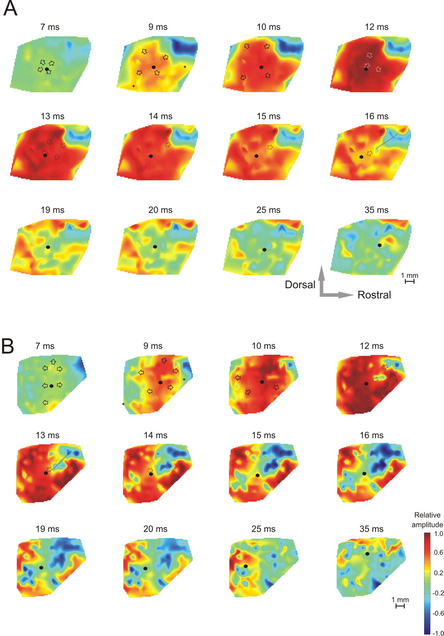
A, B, Example of propagating cortical waves and their variability demonstrated using normalized amplitudes in two congenitally deaf animals. The crosses localize the dorsal ends of the posterior and anterior ectosylvian sulcus; the arrows indicate the direction of motion of the propagating wave from the given frame to the following one. The dashed arrows are used to indicate where activity retracts, and the hexagon locates the position of the center of gravity. For movies of the propagating waves, see supplemental material (available at www.jneurosci.org).
The maximum velocity of the propagating waves was not significantly different from hearing controls (two-tailed Wilcoxon–Mann–Whitney's test, α = 0.05). The center of gravity exhibited a characteristic translation across the cortex during both contralateral and ipsilateral stimulation. A trajectory of the center of gravity was computed for every animal, and then was transposed to the same absolute position and averaged over all hearing and deaf animals (Fig. 7). In these mean trajectories, HCs showed a movement in both the rostrocaudal and dorsoventral directions. In hearing controls, the length of the COG trajectory within the first 20 ms (contralateral stimulation) was almost double that of deaf animals (12.2 ± 2.0 mm in HCs vs 6.9 ± 2.9 mm in CDCs; two-tailed Wilcoxon–Mann–Whitney's test, p = 0.021). When comparing the coordinates separately, a significant decrease in the caudorostral extent of the trajectory was observed in deaf animals when compared with HCs in the first 20 ms after stimulus (two-tailed Wilcoxon–Mann–Whitney's test, p = 0.013). In total, the whole trajectory was displaced in average by 0.7 mm caudally and 0.5 mm ventrally in deaf animals. Finally, the trajectories obtained with contralateral and ipsilateral stimulation were more similar in deaf animals. The median Euclidean distance between the center of gravity of the map obtained with contralateral stimulation and that with ipsilateral stimulation within 5–20 ms after stimulus was significantly larger in HCs than in CDCs (Fig. 7E) (median, 536 μm in HCs vs 251 μm in deaf animals; Wilcoxon–Mann–Whitney's test, p < 0.001).

Grand mean trajectories of the center of gravity computed from the normalized activation maps. A, In HCs with contralateral stimulation, the center of gravity moves first rostrally and later caudally, to finally return back rostrally. B, With ipsilateral stimulation, the rostral movement is less well expressed. C, D, In CDCs, the trajectory was shorter (for details, see Results). E, Distances between the center of gravity computed for contralateral and ipsilateral stimulation within 5–20 ms after stimulus. The distance of COG is significantly smaller in CDCs compared with HCs, demonstrating that activation maps with contralateral and ipsilateral stimulation are more similar in the former group.
Aural dominance
The microdynamics of the data demonstrated pronounced changes in aural representation in deaf animals. The hot spots evoked by contralateral and by ipsilateral stimulation overlapped well in deaf animals, as they did in HCs (Fig. 8C,D). However, the activation maps expressed in terms of contralaterality and ipsilaterality indices demonstrated differences between deaf cats and HCs: although the patchy profile of contralaterality index distribution was similar to that obtained from HCs, the patches with higher ipsilaterality and contralaterality indices overlapped more than in HCs (Figs. 8A, 10) (compare Fig. 4A). To test whether there was also a general quantitative difference, maximal contralaterality indices (in time) for each recording position were determined, the mean index over space for each animal was computed, and these means were compared between individual animals. The deaf cats had a significantly smaller averaged contralaterality index (HCs, 0.77 ± 0.02; CDCs, 0.64 ± 0.05; two-tailed t test, p = 0.0038). This was attributable to a tendency for larger ipsilateral responses in deaf animals (controls, 282 ± 59 μV; deaf, 354 ± 274 μV; two-tailed Wilcoxon–Mann–Whitney's test, p = 0.56). The absence of the latter significance was attributable to interindividual variability of LFP amplitudes, which the CI compensates for. The LFPs from CoS had a similar morphology to those of IpS in all deaf animals (Fig. 8B). This was also the case for the rostral part of the auditory cortex, where a prominent difference in the morphology was observed in HCs. This finding further demonstrates the reduced specificity for the contralateral ear in deaf animals.

Aural specificity of cortical responses in a deaf animal (the same animal as in Figure 5). A, Snapshots of contralaterality measures at different poststimulus times. A remarkable similarity of the contralaterality and ipsilaterality shows up, demonstrating that cortical topology has changed in deafness (compare with the hearing controls in Fig. 4). B, Morphology of LFPs with contralateral stimulation (blue) and ipsilateral stimulation (red) at different recording positions. Note the similarity in the morphology and peak latency of the LFPs at most positions. For a map of recording positions, see Figure 5. C, Overlay of the amplitude profile obtained with contralateral stimulation (height–profile) and ipsilateral stimulation (color). In deaf animals also, the hot spots with contralateral and ipsilateral stimulation can be seen to overlay well (compare Fig. 4). D, The relationship between the amplitudes of ipsilaterally and contralaterally evoked Pa components.
To further assess this aspect, the peak latency of the first positive component of the LFP (Pa) was plotted as a function of the amplitude of this peak (Fig. 9A,B). In HCs (Fig. 9A), a prominent difference with contralateral and ipsilateral stimulation showed up in all animals. However, in CDCs (Fig. 9B), these profiles were much more similar. The aural differences in latencies were significant in all hearing controls (paired two-tailed t test, value of p in the range between ≪0.001 and 0.039) and nonsignificant in all CDCs (value of p in the range between 0.40 and 0.80). Pooled data from all HCs demonstrated a mean peak latency of 12.6 ± 2.9 ms for CoS and 13.9 ± 3.5 ms for IpS. In CDCs, the peak latency for CoS was 13.5 ± 3.0 ms and for IpS 13.5 ± 3.4 ms. All differences of peak latencies between CoS and IpS were consequently pooled and compared (Fig. 8C). A mean difference of 1.43 ± 3.73 ms was obtained for all HCs and −0.16 ± 3.42 ms for all CD animals (positive values mean smaller latencies with CoS) (cf. Phillips and Irvine, 1983; Vischer et al., 1997; Shepherd et al., 1999). HCs showed shorter latencies with CoS than with IpS (Fig. 9C) (two-tailed Wilcoxon–Mann–Whitney's test, p < 0.001), and this difference disappeared in CDCs. This finding clearly demonstrates a deterioration of contralateral specificity in CDCs, further supported by the smeared dichotomy of contralaterality and ipsilaterality in CDCs (Fig. 10).

Amplitude–latency relationships of component Pa with stimulation at the contralateral and the ipsilateral ear. A, Controls demonstrate a complex relationship between latencies and amplitudes, with a prominent difference in latency distribution with contralateral and ipsilateral stimulation. On average, contralateral responses have shorter latencies. B, In congenitally deaf animals, these differences are less pronounced; amplitude–latency relationships for contralateral and ipsilateral stimulation are similar. Also, the range of latencies is smaller. C, Statistical comparison of peak latencies in hearing and deaf animals. Controls demonstrate shorter peak latencies with contralateral stimulation. In deaf animals, latencies are not different. ***p < 0.001.

Comparison of laterality measures in the remaining three hearing and deaf animals. Shown are snapshots at latencies when high indices were distributed over the largest cortical region. A, A dichotomy of contralaterality and ipsilaterality index with respect to cortical position is clearly discernible in hearing controls: In the rostral part of A1, high contralaterality is found, documenting a large difference in amplitude between ipsilaterally evoked and contralaterally evoked LFPs. In the caudal part of the investigated cortical region, similar LFP amplitudes for ipsilateral and contralateral stimulation (i.e., the largest ipsilaterality indices) were found. B, In deaf animals, this dichotomy disappeared.
To quantify the morphological difference of LFPs obtained with contralateral and ipsilateral stimulation, a dissimilarity index was computed within the hot spots. In HCs, HS1 had a significantly higher dissimilarity index than HS3 (Fig. 11) (two-tailed t test, p = 0.00036). In contrast, deaf animals showed no difference in dissimilarity index between the hot spots. CDCs had a significantly higher dissimilarity index in HS3 than HCs (two-tailed t test, p = 0.007). Consequently, the caudorostral binaural organization is significantly blurred in congenital auditory deprivation.

The profile of the dissimilarity index in controls (black bars). A smaller dissimilarity index was found in HS3 than in HS1. This difference disappeared in deaf cats (gray bars). Error bars indicate SD. **p < 0.01; ***p < 0.001.
Discussion
This study revealed fast evoked cortical propagating waves using electrophysiological methods and for the first time demonstrated that hearing experience significantly affects these waves. In deafness, propagating waves had less spatiotemporal fine structure, showing a more synchronized cortical activation. Furthermore, cortical contralateral dominance was compromised in congenital deafness: propagating waves and amplitude–latency relationships showed smaller aural differences, contralaterality index diminished, and field A1 lost its segregation into specific contralateral and ipsilateral regions.
Hearing controls
The general pattern of cortical activation in controls corresponds well to previous studies: the observed HS1 and HS2 correspond in location to the representation of the electrostimulated part of the auditory nerve [compare Imig and Reale (1980) and Reale and Imig (1980) with Kral et al. (1998)] (Dinse et al., 1997; Raggio and Schreiner, 1999; Bierer and Middlebrooks, 2002; Kral et al., 2006). HS1 includes the expected border between A1 and AAF (Knight, 1977; Phillips and Irvine, 1982; Schreiner and Urbas, 1986). At this spot, the cortical propagating wave broke apart into two wavefronts, one traveling caudally (through A1) and one rostrally (through AAF). As the tonotopic gradient of A1 and AAF is reversed and the unit latencies are similar (Knight, 1977; Phillips and Irvine, 1982; Schreiner and Urbas, 1986), the breakup of the propagating wave would be expected at the A1–AAF border, provided the wave initiated at the high-frequency representation and propagated to the low-frequency representation in both fields. The central narrow line in its caudal part likely corresponds to the “high-threshold ridge” observed in unit activity with CI stimulation (Raggio and Schreiner, 1999). The pattern of HS1 and HS2 corresponds well to the pattern of feline callosal connections (Imig and Reale, 1981).
Previous studies described propagating waves along the cortical isofrequency stripes (Song et al., 2006) (cf. Mendelson et al., 1997). In the present study, CI stimulation also evoked cortical propagating waves progressing in dorsal and ventral directions (along isofrequency stripes). Normalization of the amplitudes uncovered additional components propagating in the caudorostral direction. Pure tone stimulation (Harel et al., 2000; Versnel et al., 2002; Ojima et al., 2005; Song et al., 2006) might have limited the spread of cortical activation in previous optical imaging studies. The waves described here extended well outside the representation of the electrostimulated region in the cochlea (HS1 and HS2). A spread of the wave over the whole field A1 could be essential for integration of stimulus properties represented at distant parts of A1. Because the LFPs outside the hot spots had small amplitude, this cortical wave is assumed to be insufficient to drive all neurons above their threshold, but it provides synaptic input also for neurons outside of the hot spots.
Evoked waves recruiting the whole sensory area are consistent with findings from other sensory systems (Arieli et al., 1996; Petersen et al., 2003; Benucci et al., 2007). A pattern of initial (primary) and reflection waves similar to those of the present study has been described in the visual cortex using voltage-sensitive dyes (Xu et al., 2007), whereas reflection waves were more variable than primary waves. A cochlear traveling wave cannot be the reason for the cortical waves observed here, because hair cells have been destroyed at the beginning of the present experiments. The waves most likely represent a cortical phenomenon (Song et al., 2006) with thalamic contributions. Unfortunately, thalamic and cortical phenomena cannot be distinguished by the present methodology. Future research will show how the propagating waves depend on exact stimulus features.
The observed wave was very fast (∼500 μm/ms) and appeared with a short latency (cf. Song et al., 2006). Such a fast wave is of significance, because its spatiotemporal pattern falls into the integration window of neuronal processing and consequently can be made use of computationally. The long time course observed with intrinsic optical methods is most likely attributable to the delay between neural and vascular reactions.
In hearing controls, propagating waves differed with contralateral and ipsilateral stimulation. Contralateral dominance of these waves was the consequence of differences in morphology of individual LFPs between contralateral and ipsilateral stimulation. These are attributable to differences in their generators in the depths of the auditory cortex (for review, see Mitzdorf, 1985; Kral and Eggermont, 2007). Both the direction of transmembrane currents as well as their location within the cortical column determine the polarity of the LFPs recorded at the cortical surface. A difference in morphology of LFPs results from differences in the pattern of synaptic currents in the underlying cortical column. If the surface-recorded LFPs are very similar for CoS and IpS, the aural convergence most likely takes place subcortically (cf. Nelken et al., 2008). However, a difference in morphology of the LFPs demonstrates a different activation of the cortical column, and hence a difference in cortical input and/or processing of the aural inputs at the recording site. This demonstrates a “cortical contribution” to aural-specific processing.
Higher dissimilarity of LFPs evoked by contralateral and ipsilateral stimulation in HS1 and HS2 (compared with HS3) thus demonstrates more pronounced “cortical” aural-specific processing in the rostral part of A1 in hearing cats. Also, callosal connections are more extensive in the rostral part of A1 (i.e., in the high-frequency representation) (Imig and Brugge, 1978; Bozhko and Slepchenko, 1988). Because of the acoustic shadow of the head, a coherent representation of space throughout the midline requires callosal interactions (Imig and Reale, 1980; Imig et al., 1986; Poirier et al., 1995). This is of less significance in the lower frequency range, in which no head shadow exists (<3–6 kHz for the cat). The lower frequency range is represented in the few millimeters rostral from PES, where HS3 (containing similar morphology of LFPs) was found. The high dissimilarity of LFPs in AAF could be explained by preferential connections to “contralateral-dominant suppression columns” in A1 (Imig and Reale, 1981; Phillips and Irvine, 1982).
The present data further demonstrated a patchy aural representation in field A1 (patch sizes of ∼1000 μm). Discontinuous aural representation (Imig and Reale, 1980; Middlebrooks and Zook, 1983) is known to relate to different parallel thalamocorticothalamic circuits (Velenovsky et al., 2003). However, the organization of the contralaterality index did not include stripes parallel to the tonotopic axis (“binaural bands”), as some studies have suggested (Middlebrooks and Zook, 1983). The existence of “bands” has been in fact an extrapolation from recordings within smaller patches of cortical tissue. Although we did not investigate binaural interactions per se, the present data with mapping of the whole field A1 show that cortical aural organization corresponds more to patches than bands [for similar implications, see Reale and Kettner (1986) and Nelken et al. (2008)].
Congenitally deaf animals
The present study demonstrated that the cortical propagating waves are significantly shaped by auditory experience. The trajectories of the propagating waves were significantly shorter in CDCs. At the same time, neither the extent of the positive activated area nor the propagation velocity was significantly different from HCs. This implies that, in CDCs, the activity propagated more synchronously in different directions, instead of giving rise to distinct propagating waves.
CDCs additionally showed less pronounced differences in activation patterns obtained with contralateral and ipsilateral stimulation. We observed a decrease in aural dominance and changes in the pattern of aural representation in CDCs. Changes in aural representation have been demonstrated after monaural neonatal cochlear ablation (Kitzes and Semple, 1985; Moore and Kitzes, 1985; Reale et al., 1987; McMullen and Glaser, 1988; McMullen et al., 1988). The present study extends these observations by demonstrating that contralateral dominance is the consequence of “normal” hearing experience beyond balanced aural input. As aural representation is reorganized on the way from thalamus to cortex (Middlebrooks and Zook, 1983), this finding further indicates a deficit in cortical processing. Deterioration of cortical processing is further supported by the partial disappearance of the difference in LFPs with contralateral and ipsilateral stimulation and the above-described changes in propagating waves in CDCs.
Only minor effects of binaural neonatal deafening on aural representation could be demonstrated in the midbrain (Shepherd et al., 1999), contrasting with the present findings in the auditory cortex. Binaural congenital auditory deprivation thus affects more the patterning of cortical neuronal networks, whereas the analysis established at lower levels of auditory system is rudimentarily preserved. The development of auditory cortex continues up to the age of sexual maturity (Brugge et al., 1988; Eggermont, 1996; Kral et al., 2005) and depends on auditory experience (Kral et al., 2005). Therefore, the susceptibility of cortical circuits to the absence of sensory input is higher than that of subcortical networks.
The cortical representation of auditory space is unknown. The spatial location is coded by many broadly tuned neurons in a distributed manner (Middlebrooks et al., 1994). Space might be represented by the differences in activity in two channels: the ipsilaterally sensitive and contralaterally sensitive neurons (Stecker et al., 2005). Under this assumption, the deaf individual with reduced contralateral specificity would underestimate the deviation of the sound source location relative to the midline. That would in practice correspond to a partial collapse of auditory space to midline locations.
Footnotes
-
This work was supported by Deutsche Forschungsgemeinschaft Grant KR 3370/1-1 and MedEl Company (Innsbruck, Austria). We thank Dr. C. Garnham and the anonymous reviewers for valuable comments on a previous version of this manuscript. Antonia Reimer initiated the work on propagating waves in acoustically stimulated rats in the laboratory of A.K. We thank Drs. A. Haemisch and B. Tiemann for the breeding of congenitally deaf cats.
- Correspondence should be addressed to Dr. Andrej Kral, Laboratory of Auditory Neuroscience, Department of Neurophysiology and Pathophysiology, University Medical Center Hamburg–Eppendorf, Martinistrasse 52, 20246 Hamburg, Germany. a.kral{at}uke.de
References
- Arieli et al., 1996.↵
- Behrendt, 1999.↵
- Benucci et al., 2007.↵
- Bierer and Middlebrooks, 2002.↵
- Bozhko and Slepchenko, 1988.↵
- Brugge et al., 1988.↵
- Destexhe et al., 1999.↵
- Dinse et al., 1997.↵
- Dodson and Mohuiddin, 2000.↵
- Eggermont, 1996.↵
- Harel et al., 2000.↵
- Harrison et al., 1998.↵
- Hartmann et al., 1984.↵
- Heid et al., 1998.↵
- Hess and Scheich, 1996.↵
- Imig and Brugge, 1978.↵
- Imig and Reale, 1980.↵
- Imig and Reale, 1981.↵
- Imig et al., 1986.↵
- Kitzes and Semple, 1985.↵
- Knight, 1977.↵
- Kral and Eggermont, 2007.↵
- Kral et al., 1998.↵
- Kral et al., 1999.↵
- Kral et al., 2002.↵
- Kral et al., 2005.↵
- Kral et al., 2006.↵
- Leake et al., 1999.↵
- Lee and Winer, 2008a.↵
- Lee and Winer, 2008b.↵
- Massey and Denton, 1993.↵
- McMullen and de Venecia, 1993.↵
- McMullen and Glaser, 1988.↵
- McMullen et al., 1988.↵
- Mendelson et al., 1997.↵
- Merzenich et al., 1975.↵
- Middlebrooks and Zook, 1983.↵
- Middlebrooks et al., 1994.↵
- Mitzdorf, 1985.↵
- Moore and Kitzes, 1985.↵
- Nelken et al., 2004.↵
- Nelken et al., 2008.↵
- Ojima et al., 2005.↵
- Petersen et al., 2003.↵
- Phillips and Irvine, 1982.↵
- Phillips and Irvine, 1983.↵
- Poirier et al., 1995.↵
- Raggio and Schreiner, 1999.↵
- Reale and Imig, 1980.↵
- Reale and Kettner, 1986.↵
- Reale et al., 1987.↵
- Sachs, 1968.↵
- Schreiner and Urbas, 1986.↵
- Sharon and Grinvald, 2002.↵
- Shepherd et al., 1999.↵
- Song et al., 2006.↵
- Spitzer et al., 2001.↵
- Stecker et al., 2005.↵
- Velenovsky et al., 2003.↵
- Versnel et al., 2002.↵
- Vischer et al., 1997.↵
- Xu et al., 2007.↵


