

Abstract
Propagating neural activity in the developing mammalian retina is required for the normal patterning of retinothalamic connections. This activity exhibits a complex spatiotemporal pattern of initiation, propagation, and termination. Here, we discuss the behavior of a model of the developing retina using a combination of simulation and analytic calculation. Our model produces spatially and temporally restricted waves without requiring inhibition, consistent with the early depolarizing action of neurotransmitters in the retina. We find that highly correlated, temporally regular, and spatially restricted activity occurs over a range of network parameters; this ensures that such spatiotemporal patterns can be produced robustly by immature neural networks in which synaptic transmission by individual neurons may be unreliable. Wider variation of these parameters, however, results in several different regimes of wave behavior. We also present evidence that wave properties are locally determined by a single variable, the fraction of recruitable (i.e., nonrefractory) cells within the dendritic field of a retinal neuron. From this perspective, a given local area’s ability to support waves with a wide range of propagation velocities—as observed in experiment—reflects the variability in the local state of excitability of that area. This prediction is supported by whole-cell voltage-clamp recordings, which measure significant wave-to-wave variability in the amount of synaptic input a cell receives when it participates in a wave. This approach to describing the developing retina provides unique insight into how the organization of a neural circuit can lead to the generation of complex correlated activity patterns.
An emergent property of large neuronal networks in the developing and mature brain is the generation of correlated activity, which often arises via the propagation of excitation between neighboring cells. For instance, rhythmic spontaneous activity has been reported throughout the developing nervous system (Yuste, 1997), including the neocortex (Yuste et al., 1992; Kandler, 1997; Schwartz et al., 1998), hippocampus (Leinekugel et al., 1997; Garaschuk et al., 1998), spinal cord (O’Donovan et al., 1994; O’Donovan and Chub, 1997), and retina. In developing retina, retinal ganglion cells generate spontaneous bursts of action potentials (Galli and Maffei, 1988) that propagate across the ganglion cell layer (Meister et al., 1991; Copenhagen, 1996). Recently, it was demonstrated that interocular competition driven by the spontaneous action potentials in retinal ganglion cells is required for the normal patterning of retinogeniculate connections (Penn et al., 1998). The role that the spatiotemporal properties of the retinal waves play in the patterning of early connections in the retina and throughout the developing visual system, however, remains to be determined.
The spatiotemporal properties of retinal waves are well characterized by fluorescence imaging (Feller et al., 1996, 1997), and their dynamics are shaped by events that occur over long time scales (minutes) and large spatial scales (hundreds of micrometers). Retinal waves initiate at random locations in the retinal ganglion cell layer and propagate with a highly varying wavefront velocity between 200 and 600 μm/sec. They propagate over large regions of tissue encompassing hundreds to thousands of cells and terminate on distinct but nonrepeating propagation boundaries, which are defined in part by local regions of tissue included in previous waves. How the cellular properties of the individual neurons that constitute the spontaneously active circuit affect these macroscopic properties is the subject of current experiments (for review, see Copenhagen, 1996).
To address this issue, we developed a computational model of the developing retina that is based on the system-level properties of the spontaneous activity observed, rather than on the detailed biophysical properties of the cells that constitute the underlying circuitry. Previously, we have shown that a coarse-grained model of the immature retinal circuitry can reproduce the spatiotemporal properties of the retinal waves (Feller et al., 1997). Fundamental properties of this model are spontaneous random activity and a long intrinsic refractory period in individual cells. Here, we describe how the resulting dynamics of the local circuitry combine to produce the distinct spatiotemporal properties observed. Waves are initiated when a sufficient number of spontaneous events occurs in a local region in a given time interval, and waves terminate when they encounter areas with a high number of refractory cells. We explore several different regimes of wave behavior of the model, which are found by manipulating several of the model’s parameters. These distinct regimes reproduce the altered spatiotemporal properties of waves seen via pharmacological manipulations and demonstrate how the variation of cellular parameters can lead to dramatic changes in wave propagation properties.
We also present evidence that wave initiation and propagation properties are governed locally by a single dynamical variable, the local fraction of recruitable (i.e., nonrefractory) cells. The complexity of individual wave events, which propagate irregularly with large fluctuations in wave speed, arises from variations in this local population variable; as a wave encounters regions with different fractions of recruitable cells, its propagation velocity changes, possibly halting where the fraction is too low to support further propagation. The local fraction of recruitable cells evolves over longer time scales than do individual wave events, with dynamics influenced by the parameters of the model. We describe how the distinct spatiotemporal properties of the spontaneous activity observed in the developing retina arise from these dynamics, as well as how the different behaviors seen in simulation emerge via different choices of model parameters. Finally, we present data from voltage-clamp recordings of several different cell types in the retina, which provide evidence of these underlying dynamics.
MATERIALS AND METHODS
Retinal model. This simulation of the two-layer readout model was implemented using Gnu C++ and Cray C++ on several different computers (Linux Intel machines, Linux alpha machines, and a Cray T3E). The amacrine cell layer in the simulation (see Fig.1C) is a 64 × 48 honeycomb array, and the ganglion cell layer is an overlapping 128 × 96 honeycomb array.
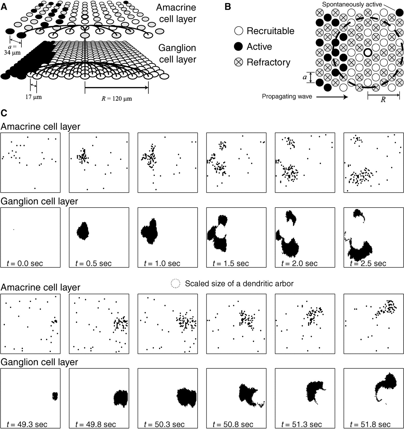
Schematic of the retinal model. A, The model consists of two overlapping cell layers, the amacrine cell layer and the ganglion cell layer, arranged in a hexagonal array. The lattice spacing of amacrine cells is given by a = 34 μm, and the lattice spacing of ganglion cells is one-half that value. An active amacrine cell stimulates neighboring amacrine cells and ganglion cells over a distance of R = 120 μm (connections are shown by dark lines). A representative state of the model is pictured, with active cells coloredblack, recruitable cells white, and refractory cells gray. As a result of the connectivity, a wave propagating in the amacrine cell layer (from theleft) only includes a fraction of the total number of amacrine cells, but the resulting wave in the ganglion cell layer is contiguous. B, The rules governing wave propagation in the amacrine cell layer are illustrated by picturing a representative state. A wave composed of active amacrine cells (black) is propagating from left to right. Refractory cells (gray with anX) are unable to participate. Recruitable cells (white) can become active by either being stimulated above threshold θ or becoming spontaneously active with probabilityp. An example recruitable cell (middle white circle with dark outline) will become active in the next time step if the number of active cells within its input radius (large dashed gray circle) exceeds the threshold θ. C, Twelve frames from the simulation picturing active amacrine cells (first and third rows) and active ganglion cells (second andfourth rows) at 0.5 sec intervals for two consecutive waves 49.3 sec apart are shown. Each frame corresponds to 1.9 mm × 1.6 mm of the retina; the size of a dendritic arbor at this scale is shown as a dashed circle.
In total, this model is completely specified by 10 parameters (described in the text), which fall into three categories. The first category represents fixed parameters and includes n (the cell density in the amacrine cell layer), R (the input radius), Δt (the elementary time step of the simulation),TF (the firing time), andTR (the average intrinsic cellular refractory period). These parameters are derived either from experimentally measured quantities or fundamental assumptions about the nature of our simulation. The second category of parameters is introduced to have realistic behavior of our system-level model and mostly arises via the coarse-graining assumptions. In this category are ΔTR (the variation in refractory periods), ΔC (the variation in input strength), and θG (the ganglion cell threshold). Small variations of these parameters have a negligible effect on the behavior of the model. Finally, the third category includes p (the rate of spontaneous amacrine cell activity) and θ (the amacrine cell threshold). These parameters are not experimentally determined and have strong effects on the behavior of the model. The simulation is studied for a wide range of these parameters in Figure2.

Behavior of the model over parameter space.A, The average interwave interval is shown as a function of model parameters p and θ. The interwave interval is a measure of the periodicity of wave activity through a given region of the retina. The full retinal simulation was run for 100 simulated minutes (n = 2) for each choice of parameter values; <10 waves occur for high threshold (θ > 4;black), and the average interwave interval is small (<30 sec between waves) for low threshold (θ < 2;white). B, Average domain size is shown as a function of model parameters p and θ. The average domain size was recorded from the same simulations shown inA, where again black represents regions where <10 waves occurred. Large waves (white) occur for small values of the spontaneous initiation rate p, and the average domain size gets smaller as p is raised.C, Data shown in A and Bis used to produce a phase diagram that distinguishes between qualitatively different regimes of wave behavior. (See Results for more details.) Video attachment, Five movies of the retinal stimulation, each representing a different point in parameter space, can be downloaded from http://marichal.berkeley.edu/jneuro. Movies show the state of the amacrine and ganglion cell layers over the course of 1 min, played in real time.
Model parameters in the first category have been estimated for the retina using previously published physiology and pharmacology results. Waves require cholinergic synaptic transmission (Feller et al., 1996) (see Results), so the cell density used corresponds to the measured density of cholinergic amacrine cells in the developing retina (called starburst cells), given approximately by n = 1000 cells/mm2 (Feller et al., 1996). The input radius of these cells is estimated to be R = 125 μm, which is consistent both with anatomical measurements and the typical scale of the retinal waves (Feller et al., 1997) (also see Figs.2A, 6A). The time interval between the activity of one cell and the subsequent stimulation of its neighbors is on the order of the cellular integration time and thus is estimated to be Δt = 100 msec (Meister et al., 1991;Wong et al., 1993). While consistent with cellular integration time scales, ultimately Δt is chosen to reproduce the experimentally measured wavefront propagation speeds. The firing time is estimated from voltage-clamp recordings of ganglion cells, which reveal large inward currents during wave events that last on the order of 1 sec (Feller et al., 1996). As a result, we setTF = 1 sec. Finally, the average refractory period is set to TR = 120 sec, which is determined by the experimentally measured peak in the interwave interval distribution, as described in Feller et al. (1997).
The model parameters of the second category are not experimentally determined. However, substantial variation of these parameters (up to a factor of two) has a negligible effect of the simulation behavior. Variability in the cellular refractory period is necessary to prevent synchronization between cells in the model, and we use ΔTR = 30 sec. Variability in input strength is necessary to prevent the unrealistic quantization of inputs onto a given cell, and ΔC = 20% of the mean input strength (which is set to unity). The ganglion cell threshold is chosen so that correlated activity (i.e., waves) in the amacrine cell layer stimulates activity in the ganglion cell layer, but uncorrelated amacrine cell activity does not. We set θG = 2θ.
The spatiotemporal properties of the model for other choices of the free parameters are studied in Figure 2. Unless otherwise specified, the two free parameters of the model, p (the rate of spontaneous amacrine cell activity) and θ (the amacrine cell threshold in units of input strength), are fixed at the following values: p = 0.03 sec−1, and θ = 3.5, such that the simulated waves have the same properties as those observed in experiment (Feller et al., 1997).
Simulation of wave propagation. A strip of 256 × 56 neurons, arranged in a hexagonal array, was used for the simulation of wave propagation pictured in Figure3A, with the input radius and cell densities discussed above. All cells within a distanceR are reciprocally coupled, and the top and bottom edges of the array are coupled together using a periodic boundary condition. Finally, recruitable cells are assigned with probability f; the remaining fraction, 1 − f, are assumed to be refractory at the time of the wave.

Wavefront velocity is governed by a single parameter. A, Simulation of the amacrine cell layer under restricted dynamics. The cell layer is started in a state with a randomly selected fraction f of cells assigned to be recruitable, and the remaining 1 − f fraction is assigned to be refractory for the duration of the simulation. Spontaneous activity is suppressed, and a wave is initiated att = 0 and allowed to propagate across the cell array. A snapshot of the state of the model after 9 sec forf = 0.3 (top), 0.4 (middle), and 0.5 (bottom) is shown with the active cells in white. Neurons stimulated above threshold are active for TF = 1 sec and then are inactive for the duration of the simulation. The gray circle shows the input radius of an individual cell.B, The wavefront velocity as a function off. Results from the simulation are shown asfilled circles, with error bars showing the variation in wavefront velocity from trial to trial. A numerical analysis of propagation velocity is shown as a dashed line, and a more detailed analytic treatment that takes into account fluctuations in the local value of f is shown as asolid line. Left axis, Velocity is scaled for values relevant to the developing retina. Right axis, Velocity is normalized byR/Δt (see Results). Bottom axis, f, the fraction of recruitable (i.e., participating) cells, is varied. Top axis, The corresponding value of the dimensionless variable α (the ratio of the number of inputs from participating cells to the threshold) is shown.
Waves were initiated on the left of the array by setting the first five columns of participating cells to be active in the first time step. The amount of stimulation that each active neuron contributes to its neighbors is selected from a normal distribution with unit mean and width ΔC = 0.2. Again, this random variation in cell coupling prevents the unrealistic quantization of cell inputs. Time evolution of this simulation is determined by calculating the amount of input each participating neuron receives from other cells within its input radius; when the sum of this input exceeds the cell threshold θ, it is made active in the next time step. The simulation time step is given by Δt = 100 msec (as in the full retinal model), and neurons stay active for TF = 1 sec = 10 simulation time steps. Note that the choices ofR and Δt restrict the propagation speed to a maximum of R/Δt = 1.2 mm/sec. Each simulation progresses until no cells are active.
Analytic model of wave evolution. The time evolution of a wave event can be predicted given the array of mesoscopic variablesf(r,t0) for all lattice sites r and the initiation pointr0. Each lattice position is assigned a propagation delay τ(r) =R/v[f(r,t0)], where the value of the velocityv[f(r,t0)] is derived from the results in Figure 3B.
The full wave evolution can then be represented on this lattice by the times that each site is active, which are calculated by finding the path from the initiation point to the site across nearest neighbors that gives the smallest summed time delays. For example, the lattice site closest to the initiation point r0 is assigned an active time of zero, and the nearest neighbors of this point are then active at the time given by the propagation delay of the initiation point τ(r0). The path that minimizes the summed time delays for all the other lattice sites depends on the distribution of time delays and can be determined via enumeration or other computational methods.
Electrophysiology. Retinal preparation and electrophysiology recordings were done as described in Feller et al. (1996). The intracellular solution contained (in mm): 100 cesium gluconate, 5 MgCl2, 1.7 CsCl, 10 EGTA, 40 HEPES, 4 ATP, 0.3 GTP, and 1 QX-314, plus 0.2–0.5% Lucifer yellow. Morphology was determined by imaging Lucifer yellow-filled cells on a scanning confocal microscope (Leica, Nussloch, Germany), with the individual layers projected onto a single plane. Ganglion cells were determined by soma size and in some cases the existence of an axon. Amacrine cells were determined by their soma size, morphology of the dendrites, and the absence of an axon heading toward the optic disk.
RESULTS
A two-layer readout model of the developing retina reproduces spatiotemporal properties of waves
Our model of the retinal waves seeks to explain the properties of the retinal waves on a system level, that is, over a time course of seconds and spatial scales of hundreds of micrometers. On these scales, the waves have distinct spatiotemporal properties, which set rigid constraints on the underlying circuitry responsible for the waves. In this section, we present a two-layer coarse-grained model for the wave-generating circuitry of the developing mammalian retina, based on previous work presented in Feller et al. (1997).
The circuitry of the developing retina at the ages considered [postnatal day 0 (P0)–P6 in the ferret] consists of two functioning cellular layers: the amacrine cell layer and the ganglion cell layer. Our model consists of these two cellular layers, as shown in Figure1A. Cell densities within each layer correspond to those observed experimentally: 1000 starburst amacrine cells per square millimeter (Feller et al., 1996) and 4000 retinal ganglion cells per square millimeter (Wong et al., 1995). In a hexagonal lattice, this corresponds to a lattice spacing of a = 34 μm for amacrine cells and 17 μm for ganglion cells.
In the model, wave activity propagates across the amacrine cell layer. Amacrine cells receive input from other active amacrine cells within their input radius R = 120 μm, which approximately corresponds to the size of the starburst amacrine dendritic arbor measured experimentally (Wong and Collin, 1989) (see also Fig.6A). The ganglion cell layer receives input from the amacrine cell layer, but we assume that ganglion cell activity does not feed back to the amacrine cell layer. Like amacrine cells, ganglion cells also receive input from active amacrine cells within their input radius, which is also chosen to be R = 120 μm (Ramoa et al., 1988).
The model evolves as a cellular automaton, in which the state of the model at time t + Δt is determined by updating the state at time t by a set of rules specific for each cell type. Amacrine cells can be in one of three states: recruitable, active, or refractory. If an amacrine cell is recruitable at a given time t, it can become active in the next time step for two reasons. (1) It is stimulated by a threshold amount of input θ from other active cells within its input radius, or (2) it becomes active spontaneously, which occurs with probability p per time step. The amount that a firing neighbor stimulates the cell is given by a random number selected from a normal distribution with a mean of unity and an SD given by ΔC = 0.2. (The units of this excitation are only relevant to whether the summed input exceeds the cell threshold given by θ.) After an amacrine cell is active, it stays active for its firing timeTF = 1 sec, at which point it becomes refractory. Finally, it will stay refractory for the duration of its intrinsic refractory period and then return to being recruitable. A cell’s intrinsic refractory period is fixed at the beginning of the simulation, selected from a normal distribution with meanTR = 120 sec and SD ΔTR = 40 sec.
A representative state of the amacrine cell layer at a given time step is shown in Figure 1B. A wave, consisting of active cells (black), is propagating across the array of amacrine cells from left to right. Refractory cells (gray with an X) are unable to participate in the wave. Recruitable cells (white) can be recruited in a wave, when they receive a threshold amount of excitation from active cells within their input radius. A representative recruitable cell (middle white circle with a dark outline) has five active cells within its input radius (dashed circle). If these cells provide stimulation greater than the threshold θ, this cell will become active in the next time step.
Figure 1C shows activity of the simulation at 0.5 sec intervals over the course of two waves. Note that spontaneous, uncorrelated activity in the amacrine cell layer does not show up in the ganglion cell layer, and subsequently only a fraction of amacrine cells is involved in any given wave. Activity in the ganglion cell layer (Fig. 1C, black, second andfourth rows) is a filtered representation of amacrine cell activity (black, first and third rows), and does not affect wave dynamics.
We include the ganglion cell layer in our model because our goal is ultimately to explain the retinal wave activity observed in experiment that, in both multielectrode recordings (Meister et al., 1991; Wong et al., 1993) and imaging (Feller et al., 1996), primarily corresponds to ganglion cell activity. In our model, ganglion cells have no intrinsic refractory period, nor any spontaneous excitability. They can be in one of two states: active or recruitable. They become active if a threshold number of amacrine cells (θG = 2θ) within their input radius R are active. They remain active for 1 sec (corresponding to the bursting time observed in experiment) and then go back to being recruitable. Because there is a threshold in the ganglion cell layer, only correlated amacrine cell activity will show up as a contiguous wave in the ganglion cell layer, whereas uncorrelated spontaneous firing will not show up at all. An example is shown in Figure 1A, where a sparse wave of amacrine cell activity (top, left, black circles) leads to a contiguous wave in the ganglion cell layer (bottom, left, black circles). Uncorrelated, spontaneous firing in the amacrine cell layer (top, right, black circle), however, is insufficiently dense to stimulate a wave in the amacrine cell layer and does not result in any activity in the ganglion cell layer. As discussed in Feller et al. (1997), this filtering of amacrine cell activity is what makes it possible to generate the distinct spatiotemporal properties of waves seen in imaging experiments.
Variation of model parameters leads to a wide range of spatiotemporal patterning
The spatiotemporal properties of the model were characterized by measuring two quantities that describe the activity in the ganglion cell layer: the average area covered by individual wave events and the average interval between wave events in a given region. The values for these quantities can be compared with those seen experimentally (Feller et al., 1997): average wave size = 0.298 mm2and average interwave interval = 126 sec. A more detailed analysis of the distribution of wave sizes and interwave intervals was performed in Feller et al. (1997) and demonstrates a more rigorous correspondence between the properties of activity produced by our model and that observed in experiment.
Here, we show how the statistical properties of the activity produced by the model change for a given choice of parameters. We vary the two principal free parameters of the model: the spontaneous initiation ratep and the threshold θ. All other parameters were held fixed at the values listed above. Further details regarding these parameters are given in Materials and Methods. Figure 2, Aand B, shows contour plots of the average interwave interval and average wave size as a function of these two parameters. These data are summarized in Figure 2C, which demonstrates how the variations in simulation behavior over the p–θ parameter space can be represented by a “phase diagram.”
A high threshold (θ > 4) suppresses wave activity, greatly reducing the frequency of waves (Fig. 2A, darker regions; Fig.2C, region V). A low threshold (θ < 2.5) gives rise to a high frequency of stimulated events, creating a short interwave interval (Fig. 2A, lighter areas; Fig.2C, region II). The area involved in a wave, however, depends on the spontaneous firing rate p (Fig.2B, left).
In the intermediate region (Fig.2A,B, gray areas), the average interwave interval and average wave area are strongly dependent on the choices of both p and θ. In the regime in which 1/p > TR (p< 0.01 sec−1) (Fig. 2C, region IV), that is, the average time it takes for a cell to become spontaneous active is longer than the cellular refractory period, wave initiations occur infrequently, so that the majority of cells will be recruitable when a wave encounters them. Waves will therefore propagate across the entire network. This regime describes the increase in frequency, wave propagation speeds, and wave area seen in the developing retina in the presence of forskolin (Stellwagen et al., 1998b), suggesting that forskolin, an activator of adenylyl cyclase, could be affecting the probability of spontaneous activity (perhaps via the regulation of synaptic machinery) and/or the threshold for amacrine cell activity. [A full explanation of these effects may include a reduction of the cellular refractory period TR that is not discussed here (see Stellwagen et al., 1998a).]
The regime with 1/p < TR (Fig. 2C, region I) displays spatiotemporal properties similar to those seen in the developing retina under normal physiological conditions. In this region of parameter space, only a fraction of the spontaneous activity leads to wave initiation and often will cause a region of the retina to become refractory without a wave event. The average wave size decreases as p is increased (Fig. 2B,C, region III) and increases as p is decreased. The effect on the interwave interval is the opposite; it increases for higher p and decreases when p is smaller (Fig. 2A). Experimental manipulation of threshold was accomplished by bathing the retina in solutions containing elevated levels of potassium (Feller et al., 1997). Such a manipulation in the model corresponds to decreasing θ, resulting in faster wave propagation, larger waves, and shorter interwave intervals, consistent with experimental observations (Fig.2C, left side of region I).
Movies of the retinal simulation, run at five representative points in parameter space, are available at http://marichal.berkeley.edu/jneuro. These movies demonstrate the qualitative features of the properties described by Figure 2C, corresponding to parameter values of region I (normal physiological conditions), I (high potassium), II (hyperactive waves), III (small waves), and IV (large waves, forskolin).
An analytic model describes the propagation dynamics of neural activity in the amacrine cell layer
Via the retinal model discussed above, we have demonstrated that a homogeneous, two-layer network can reproduce the complex dynamics of retinal waves, with minimal assumptions about cellular properties and connectivity. Activity in the retina propagates from initiation regions with variable wavefront velocities and shape. Over time, the areas that these waves span in the retina are nonrepeating and tile the entire retina on the scale of minutes. We find that these complicated dynamics can be understood by characterizing a local region of the retina by a single variable, the local fraction of recruitable (i.e., nonrefractory) cells, that completely governs local wave dynamics. In this section, we examine propagation within a wave and describe how local variations in the fraction of recruitable cells over the retina offer a simple explanation of the apparent complexity of individual wave events. In the next section, we show how the dynamics of this variable lead to an explanation of the distinct spatiotemporal properties of the retinal waves, in addition to the other regimes of wave behavior described in Figure 2.
We start by looking at wave propagation in the model under controlled conditions. Consider a model network consisting of a thin strip of the amacrine cell layer representing 8.7 mm × 1.6 mm of retina. For the duration of the simulation, spontaneous activity is suppressed, and a fixed randomly selected fraction of cells, f, is allowed to participate in wave propagation; the remaining fraction of cells, 1 − f, is refractory. A wave is initiated on the left side of the simulation and propagates as a linear wavefront across the model amacrine cell layer. Because our model assumes that the ganglion cell layer does not affect propagation dynamics, it is not considered here.
Snapshots of the state of the simulation (Fig. 3A, with active cells shown in white) are shown at 9 sec after the wave initiation for f = 0.3 (top), 0.4 (middle), and 0.5 (bottom). When the fraction of recruitable cells is higher, the wavefront travels more quickly (compare f = 0.5 with f = 0.3) and includes a higher density of cells. Measurements of the simulated wavefront velocities are plotted as data points in Figure3B, with error bars corresponding to the variation in velocity from trial to trial (n = 20). Belowf ∼ 0.3, waves are unable to propagate across the simulation (velocity is zero), because there is not a sufficient number of recruitable cells that can participate in the wave to excite their neighbors above threshold.
The dependence of the wavefront velocity on the fraction of recruitable cells can be understood via a simple argument. Consider a wavefront over one time step of the simulation. We wish to calculate how far it will move Δx during one time step Δt and thus determine the velocity v = Δx/Δt. All nonrefractory cells within the wave are active, and recruitable cells in front of the wave are receiving input from the cells in the wave. If a given recruitable cell’s dendritic arbor contains greater than a threshold number of active cells, it will become active in the next time step. All cells within a certain distance Δx will be stimulated above threshold, and the wavefront will thus shift forward by that amount.
We calculate Δx by considering the area of intersection between the dendritic arbor of a cell a distance x away and the wave. This area as a function of x is given by:
 Because all cells involved in the wavefront must have been recruitable, the number of active cells in the areaA(x) is nfA(x), wheren is the overall density of cells (n = 1000 mm−2 for starburst amacrine cells in the developing retina). All cells with nfA(x) ≥ θ will be part of the wavefront’s next time step; that is, the wave will move a distance Δx such that
 This equation can be solved numerically for Δx, and the wavefront velocity is then v(f) = Δx/Δt, shown in Figure 3B as adashed line. Note that Δx cannot be greater than the input radius R, meaning thatR/Δt = 1.2 mm/sec sets an upper bound on the velocity in this model. This upper limit ultimately arises from our fixed time step Δt and is an artifact of the coarse graining of our model; that is, events that occur on shorter time scales are averaged over and are not addressed by this model. It is notable, however, that in all cases considered, wavefront velocity does not approach this limit and is generally in the range of 100–500 μm/sec, consistent with experimental observations (Wong et al., 1993;Feller et al., 1997).
Propagation is unable to occur when the density of active cells is so low that the dendritic arbor of a cell sitting on the wavefront (at Δx = 0) does not have a threshold number of active cells within it. We can use the fact that its dendritic arbor intersects the wave with area A(0) = πR2/2 to show that the minimum value off for wave propagation to be possible is f* =nπR2/2θ. For the model parameters that reproduce the wave properties of the P0–P6 ferret retina, f* = 0.18.
For small values of f, simulation velocities are dominated by local fluctuations in the number of participating cells, leading to a marked deviation between the simulation results (Fig. 3B,circles) and the simple analytic calculation (dashed line). This deviation occurs because of the random selection of participating cells. Fluctuations can be seen to disrupt the wavefront of f = 0.3 (Fig. 3A), where there is close to the minimum number of cells participating in the wave. For larger values of f, these fluctuations have less effect, because small changes in f have smaller effects on the local wavefront velocity (see Fig. 3A, f = 0.5). The results of local fluctuations can be incorporated into a more complicated analytic calculation (discussed in the ), the results of which are shown as a solid line in Figure3B and fit the simulation results. Although the velocities seen in this calculation are specific to these particular conditions (i.e., a linear wavefront with f fixed), they are in close agreement with the simulation results, indicating that the analytic calculation of velocity versus f (represented by thedashed line in Fig. 3B) is accurate as a local prediction of wavefront velocity.
These results can be generalized to any network governed by similar coarse dynamics. For the general density of participating cellsn, cell threshold θ, input radius R, and elementary time step Δt, the speed of a linear wavefront depends on the single parameter α =nπR2/θ, the ratio of the number of participating cells in a given cell’s dendritic arbor to its threshold. The spatial and temporal scales of the model, given byR and Δt, simply determine the overall scaling of the propagation to appropriate distances and times. The scaled velocity as a function of α is demonstrated on the top andright axes of Figure 3B. Either a higher number of cells within a given cell’s input radius or a lower cell threshold results in an increase in α and a higher wave velocity. This effect saturates at the maximum velocityR/Δt. Below α* = 2, waves do not propagate at all. Golomb et al. (1996) have applied a similar argument to a simple analytic calculation for wavefront velocity of spindle waves in the adult thalamus.
A local network variable governs the wave properties of individual waves
This simple analytic model of wave propagation provides a basis for understanding the dynamics of waves in the developing retina. The complexity seen in simulation arises from the dynamics of the local network variable f described above, which reflects the interplay between the spontaneous activity of cells in the retina and a long cellular refractory period. Whereas the fraction of recruitable cells was fixed in the model of Figure 3, in the full retinal simulation it changes over both time and space: f →f(r,t). Thus, at a given time in any region of the retina, a fraction of cells [f(r,t)] will be able to participate in wave activity, and the remaining fraction [1 − f(r,t)] will be refractory, having recently been stimulated above threshold either by nearby cells or spontaneously. Wavefront velocities measured in the developing retina vary between 100 and 500 μm/sec (Feller et al., 1997). In our model, this corresponds to a range in the fraction of participating cells from 0.2 to 0.4 (from Fig. 3B). The complex shapes of the wavefronts and wave boundaries arise from the variability in the fraction of recruitable cellsf(r,t) across the retina, as we will demonstrate below.
The time evolution of a simulated wave can be predicted solely based on the values off(r,t0) at a timet0 just before wave initiation. This is demonstrated by the simulated wave shown in Figure4. At the time of wave initiation, a fraction of cells is recruitable, shown as white circles in Figure 4A, and thus is able to participate in a wave. The remaining cells in the array are refractory (black circles). The large circle with anX labels the location where the wave initiates, defined by the position of the first cell that is stimulated above threshold. After wave initiation, the simulated wavefront spreads out and eventually stops after 4 sec at a boundary labeled with a thick line (Fig. 4B). Thinner lines show the extent of the wave at 0.5 sec intervals as it evolves. A comparison between the two plots (Fig.4A,B) reveals that the initiation occurred in a region of high density of recruitable cells (Fig.4A, white circles), and the wave terminates in regions of low f. This behavior is thus governed by the collective variable f rather than the state of any individual cell.

The mesoscopic variablef(r,t) governs wave evolution.A, The state of cells in the simulation over an array of 48 × 48 neurons just before a wave initiation. The white circles indicate recruitable cells; the black circles are refractory cells. The large circlewith an X corresponds to the initiation point of the wave; the gray circle in the bottom rightis a typical dendritic arbor (∼42 cells). B, Contours representing the simulated wavefront at 0.5 sec intervals, where the wave boundary is shown as a thick line. Note that wave propagation is not uniform in the simulated retina and reaches thetop boundary in 1.5 sec and the bottom right boundary after 4 sec. Where the wave stalls, many contours overlap, also producing a thick line.C, The fraction of recruitable cellsf(r,t0) before wave initiation. This coarse-grained measure of the state of the retina is calculated from the cellular information in A, with grayscale values distinguishing between low f(dark) and higher f(white). Wave initiation occurs close to the maximum value shown (f = 0.28), and the boundary of the wavefront occurs aroundf(r,t0) ∼ 0.18. D, The predicted wave evolution using the coarse-grained measuref(r,t0). An analytic model using only the coarse-grained information inC and the initiation position is used to predict wave evolution, with contours again representing the wavefront at 0.5 sec intervals. The overall propagation time and the rough shape of the evolution are close to that found in the simulation, although details on a scale less than R are incorrect. Shaded areas show where coarse-graining errors on the boundary lead to the incorrect prediction of further propagation.
Using simulated waves like those shown in Figure 4B, we can test the hypothesis that the collective variablef(r,t) controls wave propagation in the simulation. Figure 4C is a contour plot off(r,t0)—defined as the fraction of recruitable cells within a distance R of the position r at time t0—showing a coarse-grained summary of the detailed cellular information contained in Figure 4A. Regions with a high density of recruitable cells are lighter, and regions with a high density of refractory cells are darker. The value of f at any point corresponds to the number of recruitable cells (Fig.4A, white circles) within the input radius R (an example is indicated by the dotted circle in Fig. 4A). By inspection, it is apparent that the wave boundary shown in Figure 4Bapproximately follows the contour given by f* = 0.18. Further correspondence between propagation in the simulation and the array of f(r,t0) is tested in Figure 4D.
Figure 4D represents the predicted wave evolution using only the information of Figure 4C and the initiation point as input. No knowledge of the states of individual cells was used. Wave evolution is predicted by assigning a delay to a lattice of points spaced at the input radius R. This delay is calculated as the time it takes a wave to travel a distanceR, given the local velocity determined byf(r,t0) using the analytic calculations of Figure 3B. The wave then spreads from point to neighboring point with these delays, until it runs into regions with f < f*. In comparison with Figure 4B, the wave shown in Figure4D has approximately the same overall shape and propagates to its boundary in the same amount of time, although the details are incorrect on scales smaller than the input radiusR. Because of the coarse graining, the waves predicted in this way often propagate past the boundaries that occur in the simulation (see Fig. 4D, shaded area), because the velocity we use to predict wave evolution [v(α)] assumes the width of the propagating wave is 2R (the diameter of a dendritic arbor). Occasionally, fingers with width < 2R, but withf > f*, occur along the wave boundaries, causing the predicted wave to be larger than the simulated one. It is clear, however, that the overall qualitative features of the time evolution are reproduced.
In addition to predicting wavefront propagation, the variablef(r,t) also modulates wave initiation in the retina. Note that the initiation point of the wave in Figure4B, also labeled by a large circle with anX in this plot, occurs in an area with high f(f = 0.3, a white region) in Figure4C. In our model, wave initiation occurs via simultaneous (i.e., within a firing time TR
) spontaneous activity of a threshold number of cells (θ) within an input arbor. The probability of this occurring during the intervalTR
is highly dependent on the total number of cells that could be spontaneously active in this arbor, that is, the number of recruitable cells fM, where M =nπR2 is the total number of cells within a cell’s dendritic arbor. The expected number of spontaneously active cells during a short time intervalTF
in a region with M cells is fpMTF
. The probability of above-threshold spontaneous excitation is given by the Poisson distribution:
 where we have assumed that the spontaneous activities of the cells in a given area are independent. This probability rises steeply from zero as a function of f (the fraction of recruitable cells), so that a small change in f can have large effects on the initiation probability.
Network properties arise from the long time scale dynamics of the fraction of recruitable cells
In addition to determining the features of individual events, the local population variable f(r,t) is also ultimately responsible for the complex spatiotemporal properties that are seen in the retina over long time scales (Feller et al., 1997). For example, although an average retinal wave occurs over the course of seconds, the interval between retinal waves in a given region is typically minutes. This interval does not arise from the dynamics of wave propagation but rather from the time development off(r,t), which evolves on a significantly slower time scale governed by the average refractory period TR . In the absence of a wave, each spatially separate region of the retina (i.e., separated by more than the size of a dendritic arbor) evolves independently as a locally recurrent network and is characterized by a mesoscopic parameterf(r,t). Waves involve the near synchronous activity of one or more of these areas.
To study the features of the time evolution of the fraction of recruitable cells in a given region, we monitoredf(r,t) over time in one region of the simulation of our retina model (Fig. 5). The fraction of recruitable cells changes in discrete jumps (corresponding to individual cells becoming refractory or recovering from their refractory state over the time steps of the model). Wave events traveling through the region are marked with a dark vertical bar (Fig. 5), and a solid horizontal line indicates f* = 0.18, below which propagation is not possible. In these time intervals, the network is refractory, and no wave events occur, even though individual cells may be recruitable. The length of time after the passage of a wave during which the local network is refractory varies from event to event (41.5 ± 21.6 sec; 266 waves) and is comparable with the observed refractory period seen in the retina, reported to be 40–50 sec (Feller et al., 1996). We distinguish this network refractory period from the intrinsic refractory periodTR (120 sec) of individual amacrine cells, which is a fixed parameter in our model.

The time evolution off(r,t) in a typical region of the simulated retina. A, The fraction of recruitable cells in an input arbor fluctuates over time, as measured over 8 min of simulation time (4 × TR
). The times when wave activity occurred are labeled with a dark vertical bar; a star indicates the wave initiated in the region. The solid horizontal line showsf*, such that the region is unable to support wave activity for f < f* (shaded areas). The dashed horizontal line shows the predicted equilibrium value of fin the absence of wave activity,
 B, A histogram of the values of f over a 100 min simulation is shown. The value of f in a given region was recorded at each time step (0.1 sec) over a 100 min simulation and analyzed. Although distributed over a range from 0 to 0.5, f is most frequently around the equilibrium value
 (thick dashed line) and the lower limit for propagation to be possible f* (thin solid line).
Three wave events occur in the time interval shown in Figure5A (equivalent to 8 simulated minutes), consistent with an average interwave interval of approximately the cellular refractory period TR
(120 sec). A wave typically incorporates all recruitable cells, sending f to zero. After a wave, f immediately begins to rise from zero because of the expiration of the refractory periods of cells that were not involved in the wave. In cases in which no wave activity occurs (e.g., Fig. 5A, 2.2–3.0 TR
),f levels off at an equilibrium value,
 , that can be calculated as follows. With no stimulated activity, a given cell will stay recruitable for an average time given by the reciprocal of the spontaneous initiation rate 1/p and will be refractory for an average time TR
. The probability that a given cell is recruitable is the same as the fraction of time it spends in the recruitable state, which, when averaged over a population, is equal to the equilibrium fraction of recruitable cells
, that can be calculated as follows. With no stimulated activity, a given cell will stay recruitable for an average time given by the reciprocal of the spontaneous initiation rate 1/p and will be refractory for an average time TR
. The probability that a given cell is recruitable is the same as the fraction of time it spends in the recruitable state, which, when averaged over a population, is equal to the equilibrium fraction of recruitable cells
 . Thus:
 which is shown as a dashed horizontal linein Figure 5A. When f =
 , the rate of spontaneous initiations is equal to the rate of refractory period expirations. Notice that, because of the near coincidence of
 and f*, the observed region occasionally becomes refractory because of random spontaneous cellular activity that is not sufficient to trigger a wave. This provides an explanation for experimental observations; although wave boundaries often coincide with regions of recent wave activity, they can also occur where there has been no recent wave activity (Feller et al., 1996, 1997).
To investigate further the dynamics of the local fraction of recruitable cells f, the value of f in each time step was recorded during a 100 min simulation, and these data were compiled into a histogram (Fig. 5B). This result shows thatf spans a large range over the course of the simulation but spends a large fraction of time concentrated around
 (thick dashed line) and f* (thin solid line). Because of the near coincidence of f* and
 , we see that a given region of the simulated retina is unable to participate in wave activity (i.e., f < f*) for 44% of the time (Fig. 5B, gray areas). This observation has implications for the distribution of wave sizes observed in the retina, because we hypothesize that wave boundaries arise when waves are incident on regions with f <f*.
Synaptic inputs onto retinal neurons support predictions of the model
Our model of the developing retina is derived from the study of the system properties of the network using low-magnification calcium imaging of thousands of neurons. From the distinct spatiotemporal properties produced by the developing retina, we have made predictions of the behavior of individual cells that make up the network. What does the model predict for cell physiology? First, our model implies that systematic differences between the synaptic input of different cell types need not exist in the retina to explain the observed wave behavior. From our model, we would expect to see a similar frequency and time course of synaptic input onto different cell types. Second, a critical feature of our model is that the fraction of cells that are recruitable in a given region varies from wave event to wave event (see Fig. 5A). Thus, we expect to see variation in the amount of synaptic input that a given cell receives during subsequent waves. We have tested these predictions using voltage-clamp recordings of several different cell types.
To examine the synaptic inputs of amacrine cells, we made recordings from newborn rabbit retinas (P0–P2), where morphological identification of the immature starburst amacrine cells is much better characterized (Zhou and Fain, 1996; Zhou, 1998). The propagation of waves recorded in the rabbit retina is qualitatively similar to that of waves seen in newborn ferret retina (M. B. Feller and C. J. Shatz, unpublished observations). In agreement with recent results reported by Zhou (1998), we found that starburst cells (n = 3) receive synaptic inputs with the same frequency and time course as those recorded from ganglion cells. We also recorded from nonstarburst amacrine cells (n = 5) that had similar synaptic input structure, although some amacrine cells had no apparent involvement in waves (n = 3). Examples of these recordings are shown in Figure6A. Although the gross characteristics of the compound PSCs associated with waves are similar—they occur with approximately the same periodicity—there is a significant amount of variability in the total synaptic input to a given cell from wave to wave. The results for three starburst amacrine cells, three unidentified amacrine cells, and six ganglion cells are summarized in Figure 6B. Each bar represents the recordings from an individual cell. The dots correspond to the temporally averaged net current measured for each PSC recorded from that cell (e.g., Fig. 6A, inset). The height of each bar is the average of all of the dots for that cell. As can be seen by the spread of the dots, each cell experiences a varying amount of input from wave to wave. These observations are consistent with the prediction of the model that the strength of this input is a measure of the local excitability of the network, which varies from wave to wave. As argued previously, such variability in the number of recruitable cells results in a variability in wavefront propagation velocities, offering an explanation for the observation that a given area of the retina can support waves with a wide range of propagation velocities (Wong et al., 1993; Feller et al., 1997).

Periodic compound PSCs measured in several cell types from P0 to P2 rabbit retina show a similar time course but receive a varying amount of synaptic input from wave to wave.A, Continuous whole-cell voltage-clamp recordings of 5 min with an expansion of 5 sec surrounding a compound PSCabove each trace are shown. Ganglion cells (top two traces) were determined by soma size; cholinergic amacrine cells (middle trace) and unidentified amacrine cells (bottom trace) were determined by soma size and morphology. Inset, A projection of a confocal image of a Lucifer yellow-filled cell corresponding to the recordings is shown. Scale bars, 25 μm.B, Each column refers to a different cell. The average net current was computed by averaging the individual PSCs over a 5 sec window and subtracting the baseline current recorded from the 5 sec preceding the PSC.
DISCUSSION
System-level properties motivate a coarse-grained approach to modeling the retinal waves
We have presented a coarse-grained model of the developing retina that reproduces the complex spatiotemporal properties of retinal waves observed in experiment. Wave propagation occurs in the amacrine cell layer, and the ganglion cell layer acts as a filter of this activity. Because the statistical properties of retinal waves occur on the time scale of minutes and across large spatial scales, our model is correspondingly coarse, i.e., describes retinal activity at a level of detail commensurate with time and length scales of the wave phenomenon. In our model, amacrine cell activity is not described by biophysical correlates such as membrane potential, action potentials, or firing rate. Instead, amacrine cells have three discrete states: recruitable, active, and refractory. Individual cells in the network act as coincidence detectors parameterized by a threshold θ; activity spreads when the number of active cells in a given region exceeds threshold, causing recruitable neighbors to become active. After being active, cells become refractory for their refractory periodTR . This treatment of cellular properties is very different from that in models of waves in other systems, such as the adult thalamus (Golomb et al., 1996; Rinzel et al., 1998), neocortex (Golomb and Amitai, 1997), hippocampus (Traub et al., 1989), and developing retina (Burgi and Grzywacz, 1994), which operate continuously in time and model the individual conductances of the cells involved. By averaging over details on this level, our model sacrifices direct correspondence with measurable cell physiology but is able to set constraints on cell connectivity and behavior based on the spatiotemporal properties of the system over much larger spatial and longer temporal scales.
Modeling the retina at this resolution is consistent with our findings that wave properties are governed by the population variablef—the fraction of recruitable cells within an input radiusR—rather than depending on the state of any individual cell. Because each retinal wave typically incorporates hundreds to thousands of cells, wave properties are determined by the distribution of cellular parameters across the population of involved cells. Our model parameterizes these distributions by their average (e.g., the average threshold relative to coupling is θ; the average refractory period is TR ). As more becomes known about the physiology of immature retinal circuits, it would be valuable to map measured properties of the cell types involved in the waves to the coarse parameters in the model.
Implication of the model on the organization of retinal circuitry
A novel feature of our model is that it produces spatially and temporally restricted excitation without any inhibition. Modeling the immature retina using only excitatory connections is consistent with the observations that ACh (Feller et al., 1996; Penn et al., 1998) and GABA (Fisher et al., 1998) are both excitatory at this age. The large variation in propagation speeds, as well as dynamic propagation boundaries, emerges in the developing retina as a consequence of the variable degree to which individual cells participate in the recurrent excitation of a wave. This is consistent with the amplitude variability in voltage-clamp (Feller et al., 1996), current-clamp (Zhou, 1998), and calcium-imaging experiments (Wong et al., 1993; Feller et al., 1996), although no quantitative comparison has been done. This explanation for wave boundaries in the developing retina contrasts with the understanding of the behavior of waves in the developing neocortex, where the propagation of excitation is dominated by localized coupling architecture and where domains of synchronous activity have repeating rather than continuously shifting boundaries (Yuste et al., 1995;Kandler and Katz, 1998).
Cellular features in our model that are necessary to explain these propagation dynamics and ultimately to reproduce the observed spatiotemporal properties are a probability p per time of becoming spontaneously active and a long cellular refractory periodTR . These cellular properties are assumed to be associated with the amacrine cell layer, because they have not been observed in the ganglion cell layer. Spontaneous activity is a necessary feature of the model to account for wave initiations, which occur when a threshold number of cells in a local region are spontaneously active. In addition, spontaneous activity ensures that some fraction of the population of amacrine cells will be refractory at any given time (as discussed above) and that this fraction will vary from location to location across the retina. Random fluctuations in the fraction of recruitable cells account for the experimental observation that sometimes waves have boundaries where there has been no recent wave activity (Feller et al., 1997). Because the local fraction of recruitable cells f determines wavefront propagation velocity—and whether the wave will propagate at all (see Fig. 3)—this variability in f across the retina results in the complex dynamics observed in the simulation.
What are the possible sources of spontaneous activity? Current-clamp recordings from amacrine and ganglion cells show no evidence of pacemaker currents that rhythmically depolarize cells (Penn et al., 1998; Zhou, 1998), as have been seen in other rhythmic circuits (for review, see Harris-Warrick et al., 1992; Luthi and McCormick, 1998). One possibility is that the pacemaker cell responsible for the waves has not yet been observed, and the amacrine and ganglion cells are both on the output side of the circuit. We consider this unlikely in view of the immaturity of other retinal cell types at these ages. A second possibility is that waves are initiated via spontaneous release of transmitter. Voltage-clamp recordings (Rorig and Grantyn, 1993; Zhou, 1998) (see Fig. 6A) reveal a substantial amount of spontaneous synaptic activity in immature ganglion and amacrine cells. There is evidence from cultured amacrine cells that, in the presence of several neuropeptides, amacrine cells experience periodic calcium influxes accompanied by depolarizations of ∼10 mV, which lead to spontaneous transmitter release (Borges et al., 1996). Ultimately, direct measurements of synaptic transmission between amacrine cells are required to elucidate the cellular mechanisms underlying this spontaneous activity.
A long cellular refractory period (120 sec) implies that wave activity will be influenced by the previous activity, because previously active cells will not be able to participate in new events until they are reset. Such a property is necessary to explain certain spatiotemporal features that have been observed experimentally, such as an observed network refractory period of 40–50 sec (Feller et al., 1996). What possible mechanisms exist for an intrinsic cellular refractory period? Long hyperpolarizing currents, which underlie the refractory period seen in thalamic spindle waves (Kim et al., 1995), have not been observed in amacrine or ganglion cells of the developing retina (Penn et al., 1998; Zhou, 1998). Furthermore, using simultaneous recordings,Zhou (1998) showed that depolarizations of amacrine cells are always timed with ganglion cell PSCs. This contradicts the behavior that we see in our model, in which only 20–25% of amacrine cells are involved in any given wave in the ganglion cell layer (see Fig. 1C); the rest are refractory. One possible resolution of this apparent discrepancy is that the ability of an amacrine cell to depolarize may not reflect the refractory state of the cell. For example, the refractory period may be determined by some sort of synaptic depression that prevents amacrine cells from releasing transmitter for a finite period of time. This sort of model has been proposed for describing the rhythmic activity seen in the developing chick spinal cord (O’Donovan and Chub, 1997; O’Donovan and Rinzel, 1997), and it is reasonable when thinking about the properties of a developing presynaptic terminal and its ability to rapidly and repeatedly release transmitter. If the refractory period of amacrine cells is reflected in their ability to release transmitter, then a cell could be depolarized but not be able to excite neighboring cells synaptically.
The developing retina is a spatially distributed excitatory network
We have shown that wave properties are governed by a local population variable, f(r,t), the fraction of recruitable amacrine cells within the input radiusR of a given location r. Here, the amacrine cell layer of the model is meant to incorporate all cells that contribute to the recurrent excitation associated with a wave. Because acetylcholine is the only agent known to be necessary for wave propagation in the ferret retina at the youngest ages studied (Feller et al., 1996; Penn et al., 1998), the model’s amacrine cell layer uses the measured cell densities and sizes of starburst amacrine cells (Feller et al., 1996). It is possible, however, that other cell types and coupling also contribute to wave activity. Indeed, as shown in Figure 6, many cell types receive synaptic inputs during a wave. In addition, although ACh seems to be the dominant excitatory neurotransmitter in the ferret retina that drives waves at the earliest ages studied (ages less than P10), GABA and glycine both act as depolarizing agents (Karne et al., 1997; Fisher et al., 1998), and gap junctions may also play a role in wave propagation (Penn et al., 1994; Catsicas et al., 1998; Wong et al., 1998).
The contributions of other cell types and modes of excitation are easily incorporated into the retinal model, because propagation properties depend not only on the density of recruitable cells (n) but also on the ratio of the number of recruitable cells to the threshold (α =nπR2/θ). Because the frequency of synaptic input during a wave seems to be independent of cell type (see Fig. 6), simply rescaling the threshold proportionately to an increase in cell density will produce the same dynamics of wave propagation. In considering the network behavior overall, however, there are two other factors to consider. First, the distribution of wave sizes, as well as their structure, is set by the range of excitatory coupling R (Feller et al., 1997). Thus, although other modes of communication between cells might exist, we expect it to be dominated by coupling over the length scale R. Second, if a larger density of cells contributes to the recurrent excitation of a wave, more averaging will result, and thus less fluctuations in the local fractions of recruitable cells [f(r,t)] are expected. Because fluctuations in f(r,t) are ultimately responsible for the complex dynamics of retinal waves, we expect the requirement of sizable fluctuations to constrain the number of independent elements that contribute to initiation and/or propagation of waves.
Without a well-defined pacemaker circuit, what determines the periodicity of the activity? Our model predicts that every local region of the retina would produce episodic quasiperiodic activity and that its regularity would arise from the population as a whole. Similar rhythmic activity, namely, periodic bursts of action potentials separated by minute-long quiescent intervals, has been seen in other developing circuits, namely, the chick spinal cord preparation (O’Donovan and Chub, 1997) and rat hippocampus (Leinekugel et al., 1997; Garaschuk et al., 1998). In both of these circuits, there are no well-defined pacemaker cells or circuits, and the activity is driven by recurrent excitatory connections between local circuit interneurons and projection neurons of the system (motoneurons in the spinal cord and pyramidal cells in the hippocampus). Given the remarkable similarities between production of activity in these circuits and that of local regions of the developing retina, it is possible that similar organizing principles underlie their respective circuitry. However, in the retina, the periodicity of a local region is influenced by the activity of neighboring regions, in addition to its own intrinsic activity. This results in the distinct spatial, as well as temporal, patterns that we observe.
Conclusion
We have shown that wave behavior can be governed by mesoscopic properties of a network and may be robust with respect to variations in the detailed biophysical properties of individual neurons. Such mechanisms could be a general strategy used by developing circuits, where coherent and synchronous activity is necessary to guide further development, but cellular properties such as synaptic transmission and connectivity are not yet fully developed. There are many examples of spontaneously active circuits comprising immature connections (seeYuste, 1997). Although these various networks can be significantly different in both connectivity as well as in the types of cells involved, their large-scale features have many similar properties, namely, correlated activity mediated by immature synapses. In fact, in the retina itself, waves are mediated by different circuits in different species and at different ages (Sernagor and Grzywacz, 1996; Sernagor and O’Donovan, 1997; Catsicas et al., 1998; Fisher et al., 1998), suggesting that a coarse-grained model can provide a useful unified description of these various networks.
ANALYTIC MODEL OF WAVEFRONT VELOCITY INCLUDING FLUCTUATIONS
Cells in the simulation that participate in wave propagation are randomly selected with probability f. Because of the random selection of recruitable cells, there will be fluctuations inflocal(r), which is averaged over an input radius, from location to location. The probability of havingN participating cells in a region containing Mcells (and thus flocal =N/M) is given by a binomial distribution:
 where M =nπR2 is the total number of cells in the dendritic arbor.
As the wave travels across each region, its velocity is determined byflocal, such that traveling a distanceR takes a timeR/v(flocal), where v(flocal) refers to the results of the analytic calculation presented in Figure3B. The velocities measured in the simulation (Fig. 3) were averaged over many trials. In many trials, the wave did not make it across the length of the simulation, meaning that the velocity for that trial was zero. The probability that a wave will stop over the distance of a dendritic arbor (2R) is given by the probability that an area will have flocal <f*, which is given by a sum of probabilities:
 In the simulation, the wave must travel a distance Land thus traverse L/2R regions of length 2R. The probability of the wave not stopping in any of these regions, thereby making it across, is given by [1 −Pstop(f)]L/2R.
Now, given that the wave does not encounter a region off < f* and thus propagates across the entire array, the average time it will take to propagate a unit distance is:
 Thus, the average velocity of propagation across a distanceL, measured over many trials, is given by:
 These results are shown in Figure 3B (solid line).
Footnotes
This work was supported by a Department of Energy LDRD-3668-27 to D.A.B. and D.S.R., an ARCS Foundation Fellowship to D.A.B., a Miller Institute Postdoctoral Fellowship to M.B.F., and National Science Foundation Grant IBN9319539, National Institutes of Health Grant MH 48108, and a grant from the Alcon Research Institute to C.J.S. This research used resources of the National Energy Research Scientific Computing Center, which is supported by the Office of Energy Research of the United States Department of Energy. C.J.S. is an Investigator of the Howard Hughes Medical Institute. We wish to thank John Rinzel for his extensive comments on this manuscript.
Correspondence should be addressed to Dr. Daniel A. Butts, Department of Physics, 366 LeConte Hall, University of California, Berkeley, CA 94720-7300. E-mail address: dbutts{at}physics.berkeley.edu
Dr. Feller’s present address: National Institutes of Health, National Institute of Neurological Disorders and Stroke, 36 Convent Drive, Bethesda, MD 20892-4156.


