

Abstract
We performed a systematic analysis of phase locking in pairs of electrically coupled neocortical fast-spiking (FS) and low-threshold-spiking (LTS) interneurons and in a conductance-based model of a pair of FS cells. Phase–response curves (PRCs) were obtained for real interneurons and the model cells. We used PRCs and the theory of weakly coupled oscillators to make predictions about phase-locking characteristics of cell pairs. Phase locking and the robustness of phase-locked states to differences in intrinsic frequencies of cells were directly examined by driving interneuron pairs through a wide range of firing frequencies.
Calculations using PRCs accurately predicted that electrical coupling robustly synchronized the firing of interneurons over all frequencies studied (FS, ∼25–80 Hz; LTS, ∼10–30 Hz). The synchronizing ability of electrical coupling and the robustness of the phase-locked states were directly dependent on the strength of coupling but not on firing frequency. The FS cell model also predicted the existence of stable antiphase firing at frequencies below ∼30 Hz, but no evidence for stable antiphase firing was found using the experimentally determined PRCs or in direct measures of phase locking in pairs of interneurons.
Despite significant differences in biophysical properties of FS and LTS cells, their phase-locking behavior was remarkably similar. The wide spikes and shallow action potential afterhyperpolarizations of interneurons, compared with the model, prohibited antiphase behavior. Electrical coupling between cortical interneurons of the same type maintained robust synchronous firing of cell pairs for up to ∼10% heterogeneity in their intrinsic frequencies.
Introduction
Neural circuitry in layer IV of rat barrel cortex includes a network of excitatory regular-spiking (RS) cells and two networks of inhibitory interneurons: fast-spiking (FS) and low-threshold-spiking (LTS) cells (Gibson et al., 1999; Beierlein et al., 2000, 2003). Paired whole-cell recordings have shown that inhibitory interneurons of the same type are electrically coupled (Galarreta and Hestrin, 1999; Gibson et al., 1999; Tamas et al., 2000; Hestrin and Galarreta, 2005) and that this coupling can promote synchronous activity (Galarreta and Hestrin, 1999; Gibson et al., 1999; Blatow et al., 2003; Chu et al., 2003; Galarreta et al., 2004; Merriam et al., 2005).
Recent theoretical work has suggested that the ability of electrical coupling to synchronize the activity of cells depends on a number of factors, including coupling strength and firing frequency (Chow and Kopell, 2000; Lewis and Rinzel, 2003; Nomura et al., 2003; Pfeuty et al., 2003; Di Garbo et al., 2005; Bem et al., 2005; Saraga et al., 2006). This theoretical work predicts that, under most conditions, electrical synapses promote synchronous activity, but they can also support antiphase activity between coupled neurons.
We recorded from electrically coupled pairs of FS and LTS cells in the rodent thalamocortical slice preparation and compared our results with those obtained in a conductance-based model of electrically coupled FS cells. We conducted a thorough experimental analysis of the effects of electrical coupling in pairs of cortical interneurons recorded simultaneously, while driving them through protocols designed to promote either synchronous or asynchronous activity. We examined phase-locking properties over a wide range of firing frequencies and coupling strengths (Gibson et al., 2005). Variation in coupling strength occurred naturally and was also controlled artificially using dynamic clamp (Sharp et al., 1993; Dorval et al., 2001; Pinto et al., 2001). We explicitly studied the robustness of phase-locked states to heterogeneities in the intrinsic frequencies of the coupled cells. We constructed phase–response curves (PRCs) (Reyes and Fetz, 1993a,b; Galán et al., 2005; Gutkin et al., 2005) for real FS and LTS cells and for the model FS cell. The PRCs, along with the theory of weakly coupled oscillators (Kuramoto, 1984; Hansel et al., 1995; Kopell and Ermentrout, 2002; Lewis and Rinzel, 2003; Pfeuty et al., 2003), were then used to obtain insight into the observed phase-locking patterns.
Materials and Methods
Slice preparation and recording.
Tissue was obtained from three different rodent strains: Sprague Dawley rats, FVB-TgN (Gad GFP) 45704 Swn mice (The Jackson Laboratory, Bar Harbor, ME), and G42/C57BL/6 mice (Z. Josh Huang, Cold Spring Harbor Laboratory, Cold Spring Harbor, NY) ages postnatal days 13–16. FVB-TgN (Gad GFP) 45704 Swn mice express green fluorescent protein (GFP) in somatostatin-expressing cells and were used to aid in the visualization of somatostatin-expressing LTS cells. G42/C57BL/6 mice express GFP in parvalbumin-positive cells and were used to aid in the visualization of parvalbumin-expressing FS cells. Thalamocortical slices (Agmon and Connors, 1991) 350–400 μm thick were prepared in ice-cold artificial CSF (ACSF). Slices were immediately transferred to 32°C ACSF for 1 h. Slices were then transferred to room temperature and kept at that temperature in the recording chamber (22.7 ± 1.4°C). ACSF was saturated with 95% O2/5% CO2 and was composed of the following (in mm): 126 NaCl, 3 KCl, 1.25 NaH2PO4, 2 MgSO4, 26 NaHCO3, 10 dextrose, and 2 CaCl2.
Patch pipettes were made from 1.5 mm glass (Sutter Instruments, Novato, CA) and filled with the following (in mm): 130 K-gluconate, 4 KCl, 2 NaCl, 10 HEPES, 10 sucrose, 0.2 EGTA, 4 ATP-Mg, 0.3 GTP-Tris, and 14 phosphocreatine-Tris (pH adjusted to 7.25 with 1 m KOH and osmolarity to 295 mOsm). Whole-cell patch recordings were obtained under infrared-differential interference contrast (IR-DIC) using a Nikon (Tokyo, Japan) E600-FN microscope. Current-clamp recordings were obtained using Axoclamp 2B amplifiers (Molecular Devices, Palo Alto, CA). Data were collected and analyzed using programs written in LabVIEW 5.0 (National Instruments, Austin, TX).
Dual whole-cell recordings from pairs of interneurons of rat and mouse barrel cortex were obtained by either selecting cells under IR-DIC with large vertically oriented somata (Amitai et al., 2002) or selecting fluorescent cells from GFP-expressing mice.
AMPA/kainate and NMDA receptors were blocked with either 2.4 mm kynurenic acid or a combination of 50 μm d-2-amino-5-phosphonovaleric acid and 20 μm 6,7-dinitroquinoxaline-2,3-dione. The presence of inhibitory synaptic connections was checked by depolarizing the postsynaptic cell while evoking action potentials in the presynaptic cell. When IPSPs were observed, GABAA-mediated inhibition was blocked by adding 50 μm picrotoxin. Drugs were obtained from Sigma (St. Louis, MO) and bath applied to the slices.
Coupling coefficient, cs.
The strength of electrical coupling between pairs of neurons was quantified using a coupling coefficient (cs) (Bennett, 1977). cs was calculated by injecting a hyperpolarizing current step into cell 1 (−500 pA, 10 trials) and dividing the amplitude of the steady-state voltage deflection produced in cell 2, ΔV2, by the amplitude of the steady-state voltage deflection in cell 1, ΔV1, i.e., cs = ΔV2/ΔV1 (Fig. 1) (Gibson et al., 1999).

Whole-cell current-clamp recordings of FS cells (left) and LTS cells (right), in layer IV of somatosensory cortex, showing their typical membrane voltage responses to current steps. A, Response of cells to suprathreshold current injections. B, Responses of electrically coupled pairs of cells to suprathreshold and hyperpolarizing currents steps injected into cell 1. The bottom set of traces show the voltage responses attributable to coupling in the second cell (cell 2).
Electrical coupling using dynamic clamp.
Three pairs of interneurons with weak or no electrical connections were artificially coupled with either analog- or software-based dynamic clamp (Sharp et al., 1993; Dorval et al., 2001; Pinto et al., 2001). Coupling was modeled as an ohmic conductance, i.e., the coupling current injected into cell j was Icoup,jk = gcoup(Vk − Vj), j,k = 1,2; j ≠ k, where Vj is the membrane potential of the jth cell.
Stimulus protocols: ramps and steps.
A firing frequency versus injected current (f–I) plot was constructed for every cell using intracellular current steps. Current steps started at −400 pA and were incremented in 50 pA steps toward more depolarizing levels until near-saturation of the firing frequency. Each step lasted 600 ms.
The f–I plots were used to construct current ramps and current steps intended to drive both cells of a simultaneously recorded cell pair through a matched range of firing frequencies. Current ramps drove both cells continuously through a range of frequencies. Current steps were used to examine interactions between the cells at different steady-state frequencies.
Current ramps started at a level below firing threshold to examine the widest possible range of frequencies. Each ramp lasted a total of 15 s. Current steps lasted 1 s each and were presented with a 5 or 10 s interstep interval. To avoid biasing the phase locking of pairs toward synchrony, the onsets of the steps presented to the two cells were offset by 6 ms.
Stimulus protocols: experimentally determined PRCs.
A small-amplitude, brief current stimulus delivered at a particular time in the firing cycle of a cell shifts the phase of the firing time of the cell (Reyes and Fetz, 1993a; Mattei and Schmied, 2002; Galán et al., 2005; Gutkin et al., 2005). Measuring these phase shifts, Δθ, attributable to stimuli presented at many (or theoretically all) different times, t, and normalizing by the amplitude, Istim, and duration, Δt, gives the PRC:
 where T is the natural firing period of the cell when unperturbed.
PRCs for FS and LTS cells recorded in vitro were constructed by using either 400 or 500 ms current steps to evoke repetitive firing at a fixed frequency. During this activity, a 2 ms, depolarizing current pulse was used to perturb the cell. The amplitude of the pulse was adjusted to produce a ∼2 mV deflection in the membrane potential when cells were at rest (Reyes and Fetz, 1993a). This was repeated in 100–150 trials for each neuron. To vary the timing (phase) at which the pulse was delivered, we used the natural variability in spike timing (i.e., jitter) during repetitive firing (for values of the variance in interspike intervals as a function of firing rate, see supplemental Fig. 1, available at www.jneurosci.org as supplemental material). The phase change produced by the pulse was calculated by the time difference between the interspike interval (ISI) of the two spikes immediately preceding the pulse and the ISI of the two spikes surrounding the pulse. The phase change, Δθ, was divided by the duration and amplitude of the stimulus and plotted against the phase of the stimulus t (i.e., the time difference between the pulse and the preceding spike) to obtain the PRC Z(t). For each PRC, the median period of the oscillations T was found, and the membrane potential for a cycle of period T was obtained [V0(t)]. Data in each PRC were binned using 1 or 2 ms bins, and the mean value of the data in each bin was computed. A least-squares fit to these mean values using a combination of sinusoids (the 0th to the second Fourier modes) was performed to obtain the fitted PRCs [Z(t)].
Data analysis.
The LTS cells in our study showed the typical spike frequency adaptation characteristic of LTS cells (Kawaguchi, 1993; Kawaguchi and Kubota, 1993; Gibson et al., 1999), whereas the FS cells showed little spike frequency adaptation with short current pulses (Kawaguchi, 1993; Kawaguchi and Kubota, 1993; Gibson et al., 1999). Current ramps were nonstationary by design, and care was taken to select a window size, for analysis, in which the spike frequency change was small. Responses evoked by stimulus ramps were divided into time windows that included 20 spikes over which the frequency was approximately stationary; the fixed number of spikes was necessary to avoid introducing a bias attributable to differences in sample size at different frequencies.
The 1 s current pulses used in our study produced a small degree of spike frequency adaptation in FS cells (Descalzo et al., 2005) and the typical spike frequency adaptation in LTS cells. The initial 100 ms of the step was not used for the analysis, eliminating much of the spike frequency adaptation observed in LTS cells (Fig. 1). For responses evoked by the current steps, the number of spikes used was set to the number that occurred during the last 900 ms of the trial having the lowest response (∼10 spikes for LTS cells; ∼20 spikes for FS cells).
Discrete cross-correlograms of action potentials for each response window were obtained by calculating the time intervals between spikes in cell 1 and cell 2, binning the intervals to generate histograms (bin size of 1 ms) and normalizing the histograms by the total number of spikes evoked in cell 1, as described by Beierlein et al. (2000). Running cross-correlograms were obtained by sequentially concatenating the correlograms for each nonoverlapping individual response window and smoothing.
A correlation coefficient of synchrony, CC0, was taken to be the peak of the running cross-correlogram in a ±5 ms interval centered at 0 ms for each cell pair. Because of the low number of spikes and relatively low jitter in the periodic firing process, three trials using the same current ramp were performed, and the average of three trials was used to obtain summary correlation data.
The correlation coefficient used here does not take into account the periodicity of the firing of the cells; therefore, circular statistics (Batschelet, 1981; Drew and Doucet, 1991) were used to obtain a more general measure of phase locking. Specifically, the mean phase difference between the cells [Φ ϵ (−π, π]] and squared vector strength R2 were calculated for the spike trains of cell pairs (for details, see Appendix). R2 is a measure of the concentration of individual phase differences around the mean Φ, i.e., it is a measurement of the variance of phase differences. R2 = 1 indicates perfect phase locking at the mean phase difference Φ, whereas R2 = 0 indicates that the individual phase differences are distributed uniformly around the circle (−π, π].
Random jitter model for phase differences between uncoupled cells.
When FS and LTS cells fire in response to prolonged depolarizing currents, there is relatively low random jitter in the ISI. Therefore, when two uncoupled cells are made to fire at the same frequency, the drift away from the initial phase difference will be slow, leading to a bias in the mean phase difference and an overestimation of R2. If a large enough sample of action potentials is used to compute the phase differences, individual phase differences will uniformly cover the circle (−π, π], R2 will be approximately 0, and the bias will have little effect on the results. However, when the sample of action potentials is small relative to the amount of jitter in the ISIs, the effect of the bias can be substantial. Thus, when assessing the effects of electrical coupling on phase locking, it is essential to know when the effects on the correlation coefficient CC0 and the square of the vector strength R2 are significant.
Standard significance tests (e.g., the Rayleigh test for R) could not be directly applied to the data, because the sample of individual phase differences is small and the individual phase differences used to calculate R2 and Φ are not sufficiently random as described above. Therefore, a random walk model was designed to determine baseline values for R2 and CC0 for pairs of uncoupled cells. The model generated pairs of spike trains with the same mean period but with spike times that varied independently because of independent random jitter. The magnitude of the jitter as a function of the mean period was experimentally determined for FS and LTS cells and for current ramps and current steps (supplemental Fig. S1, available at www.jneurosci.org as supplemental material). The mean and the variance of R2 and CC0 were computed as a function of the mean period for each condition. The model was also used to estimate the probability that uncoupled cells would appear phase locked (within ±1 ms) for a given number of spikes purely by chance. We will refer to this model as the “random jitter model.” Details of the model are provided in Appendix.
Model FS cell pair.
A model of two FS cells coupled by an electrical synapse was also studied. The intrinsic dynamics of the cell pair were identical and were governed by a conductance-based model for neocortical FS interneurons, specifically the model of Erisir et al. (1999) as modified by Jolivet et al. (2004) and Lewis and Rinzel (2004). Electrical coupling was modeled as an ohmic resistance between the cells (Bennett, 1977). The FS model equations are as follows:
 where Vj is the membrane potential (millivolts) of the jth cell, mj, hj, nj, and pj are the gating variables of the jth cell, Cm is the membrane capacitance (picofarads), gcoup is the coupling conductance (nanosiemens), and t is time (milliseconds). The functions Iionic, y∞, and τy are given by the Erisir et al. (1999) model (for a detailed description of the model, see supplemental data, available at www.jneurosci.org as supplemental material). The parameters used here were the same as those in the original Erisir et al. model except that the leakage conductance, gleak, was divided by 5 to better match the membrane time constants of cortical FS cells (Beierlein et al., 2003), and the membrane surface area was increased by a factor of 5 to better match the experimentally measured input resistance of FS cells. Īapplied is the average current applied to the cells (Iapplied,j + Iapplied,k)/2 and was used to control the intrinsic firing frequency. ΔI is the difference between the currents applied to each cell Iapplied,j − Iapplied,k and was used to control the heterogeneity between the cells.
The theory of weakly coupled oscillators and the G-function.
For weak coupling and weak heterogeneity, the theory of weakly coupled oscillators (Kuramoto, 1984; Hansel et al., 1995; Ermentrout and Kleinfeld, 2001; Kopell and Ermentrout, 2002; Lewis and Rinzel, 2003; Pfeuty et al., 2003; Galán et al., 2005) provides an equation that governs the evolution of the phase difference between the coupled cells φ. This is accomplished by using the membrane potential of the uncoupled cells during the oscillation V0(t), the corresponding phase-response curve Z(t) of the cells, and the expression of the model coupling current.
We used this theory to examine phase-locking properties in both the model FS cells and the real cortical interneurons. A brief derivation of this equation is given in the Appendix. In this derivation, the cells are assumed to have identical intrinsic properties and to fire repetitively with an intrinsic period T. Also, the electrical coupling between cells is assumed to be weak (see below), and weak heterogeneity is assumed to arise only from a small difference in their applied current ΔI. The equation governing changes in the phase difference is as follows:
 where
where
 We will refer to the function G(φ) as the “cell pair coupling function” or the G-function. There are 1:1 phase-locked states at values of φss, where gcoupG(φss) = ΔI Q, i.e., steady states of Equation 2. These phase-locked states are stable if G′(φss) < 0. Note that the 1:1 phase-locked states are only present when the intrinsic frequencies of the cells are sufficiently close, i.e., whenever |ΔI| ≤ gcoupG*/Q, where G* is local maxima of G(φ).
Results obtained using the theory of weakly coupled oscillators are only quantitatively accurate for sufficiently weak coupling and heterogeneity, but the qualitative results usually extend to moderate coupling and heterogeneity. Sufficiently weak coupling implies that the coupling conductance is at least an order of magnitude smaller than the input conductance gcoup ≪ ginput, which leads to cs ≪ 1 (based on a passive single compartment cell pair model). Note that electrical coupling between individual pairs of cortical interneurons is weak in most cases with the average coupling coefficient cs of ∼0.1 (Gibson et al., 1999) (Table 1). Also, note that, when cells are in an oscillatory mode, the minimum intrinsic membrane conductance is usually substantially greater than the resting membrane conductance. This effectively makes the coupling even weaker.
Mean cell parameters for the population of FS and LTS cells
Results
Characteristics of FS and LTS cells
Interneurons were classified as either FS (n = 40) or LTS (n = 31) based on their firing patterns (Galarreta and Hestrin, 1999; Gibson et al., 1999; Beierlein et al., 2003) (Fig. 1). Both FS and LTS cells fired periodically in response to sufficiently strong constant applied currents (Fig. 1A) (see example of f–I curve in Fig. 4A). LTS cells appeared to be able to fire at “arbitrarily” low frequencies (type I excitability), whereas FS cells rarely were able to fire regularly below ∼25–30 Hz (type II excitability) (Tateno et al., 2004). Mean maximal frequencies for FS and LTS cells were 81 ± 19 and 44 ± 9 Hz, respectively. FS cells had narrow action potentials (1.0 ± 0.2 ms) and little adaptation in their firing patterns (Kawaguchi, 1993; Kawaguchi and Kubota, 1993; Gibson et al., 1999). LTS cells had wider action potentials (1.4 ± 0.3 ms) and adapting firing patterns (Fig. 1A; Table 1) (Kawaguchi, 1993; Kawaguchi and Kubota, 1993; Gibson et al., 1999). The resting membrane potential, input resistance, spike amplitude, spike half-width, spike threshold, and high frequency were all significantly different between FS and LTS cells (p < 0.01) (Table 1).
PRCs
To further characterize FS and LTS cells, we obtained PRCs for both types of interneurons and for a conductance-based model of a neocortical FS cell. PRCs characterize the sensitivity of cells to small, brief perturbations delivered at different phases in their firing cycle and plot the phase shifts caused by the perturbations as a function of the phase at which they were delivered. PRC data were obtained for individual FS (n = 10) and LTS (n = 5) cells at various intrinsic frequencies. Figure 2, A and B, shows examples of PRCs [Z(t)] and the corresponding membrane potential [V0(t)] for a single FS cell firing at 50 and 28 Hz. These experimentally determined PRCs were similar to PRCs obtained from the model FS cells at similar frequencies (Fig. 2C,D). In both cases, the phase t = 0 is arbitrarily set to the time that the membrane potential crosses 0 mV during the upstroke of action potential. The PRCs are relatively close to 0 in the first half of the cycle (during and immediately after the action potential) and have a large positive portion in the second half of the cycle, peaking at approximately three-quarters through the cycle. This indicates that the FS cells are relatively insensitive to perturbations (attributable to applied current or current arising through coupling) in the first half of the cycle and are very sensitive to current input at phases around 3T/4. Furthermore, in the second half of the cycle, in which cells are most sensitive, the cells responded to positive current input with phase advances. As can be seen in Figure 2, the cells were more sensitive to input when they were firing at lower frequencies, i.e., the positive portion of the PRC is much larger at the lower frequencies. This corresponds to theoretical results for most neuronal models (Brown et al., 2004; Gutkin et al., 2005). PRCs for other FS and for LTS cells were similar to those described above (supplemental Figs. S2–S4, available at www.jneurosci.org as supplemental material). In general, when compared with the PRCs for LTS cells and the FS cell model, the PRCs for the real FS cells appeared to have a less distinct negative portion in the first half of the cycle and a smaller positive peak in the second half of the cycle.

PRCs and predictions using the theory of weakly coupled oscillators. A–D, Data are shown for a real FS cell firing at 50 Hz (A) and 28 Hz (B) and for the FS model cell firing at 50 Hz (C) and 25 Hz (D). Top traces show single periods of the membrane potentials (V0), and middle traces show the corresponding phase–response curves [Z(t) in units of pA−1]. For the real FS cell, multiple cycles of V0 are shown in gray, and the cycle with the median period is shown in black. For the PRCs of the real FS cell, experimental data points are shown as gray dots, averaged (binned 1 ms) data points are shown as black dots with vertical lines denoting SDs, and the fits to the data points are shown by the black curves. Bottom traces show the corresponding G-functions G(φ) for a pair of electrically coupled cells (in units of nS−1). The height of G(φ) is proportional to the coupling strength gcoup. The zeros of G(φ) indicate the phase of the phase-locked states. When the slope of G(φ) is negative at the zero, the corresponding phase-locked state is stable. Conversely, when the slope is positive, the phase-locked state is unstable. The G-functions for the “real” FS cell pair at both 50 and 28 Hz and for the model FS cell pair at 50 Hz indicate that only synchrony (φ = 0, 2π) is stable. For the model FS cell pair at 25 Hz, the G-function indicates that both the synchronous and antiphase (φ = π) states are stable.
Experimentally determined PRCs predict only synchronous activity
Using the theory of weakly coupled oscillators, the fitted PRCs Z(t), and the corresponding membrane potential fluctuations V0(t) were used to compute the cell pair coupling functions or G-functions for cell pairs with weak electrical coupling (see Materials and Methods). This enabled us to make predictions concerning the phase locking between pairs of interneurons. Figure 2, A and B (bottom), shows examples of G-functions for an FS cell firing at 28 and 50 Hz. The G-functions have zeros only at phase differences φ = 0, π, and 2π. Slopes of the G-functions generated using the experimental PRCs were always negative at φ = 0 and 2π and were always positive at π. This indicates that synchrony (φ = 0, 2π) was the only stable phase-locked state and that antiphase activity (φ = π) was always unstable. Qualitatively, the results were the same for all G-functions computed, i.e., for all real FS cells (n = 11; 28–66 Hz) and LTS cells (n = 5; 25–30 Hz) studied (supplemental Figs. S2–S4, available at www.jneurosci.org as supplemental material). That is, despite the significant differences in intrinsic properties of FS cells and LTS cells, the PRC analysis predicted the same phase-locking behavior for both cell types: only synchronous activity is stable.
As with real neocortical cells, the theory of weakly coupled oscillators showed that stable synchronous activity exists in the model FS cell pair (with identical intrinsic frequencies ΔI = 0) over the entire frequency range studied (20–90 Hz in 0.1 Hz steps). However, in contrast to the real cells, the analysis also revealed that the model cell pair supported antiphase activity at low frequencies (20–30 Hz), i.e., there was bistability. Figure 2, C and D (bottom), plots the G-functions calculated for pairs of electrically coupled model FS cells at intrinsic frequencies of 50 and 25 Hz, respectively. At 50 Hz, the G-function only has zeroes with negative slopes at 0 and 2π, indicating that only synchronous activity is stable. Conversely, the G-function at 25 Hz has a 0 with negative slope at π as well, indicating that stable antiphase activity coexists with the synchronous state. The zeros with positive slope act as boundaries separating the region of attraction for the two different stable phase-locked states. The overall phase-locking behavior of the model is shown on the bifurcation diagram in Figure 3A, which plots the phase differences φ of the phase-locked states as a function of intrinsic frequency. Only synchrony is stable at higher frequencies (>30 Hz), and there is bistability of synchronous and antiphase activity at lower frequencies (20–30 Hz).

Frequency dependence of phase locking in the model FS cell pair. A, Bifurcation diagram plotting the phase difference (φ/T) of all phase-locked states as a function of the intrinsic frequency of the cells. Solid black lines and solid gray line indicate stable synchronous and antiphase states, respectively; gray dashed lines indicate unstable phase-locked states. The stable synchronous activity exists over the entire frequency range studied (20–90 Hz). Antiphase activity is also supported at sufficiently low frequencies (<30 Hz), i.e., there is bistability at these frequencies. B, Numerical simulations of the FS model cell pair with cs of 0.08 at an intrinsic frequency of 50 Hz, showing that cells quickly evolve to a synchronous state. C, Numerical simulations of the FS model cell pair with a coupling coefficient of cs of 0.08 at an intrinsic frequency of 25 Hz. Different initial conditions can lead to synchronous activity or antiphase activity.
Direct numerical simulations of the FS cell pair model concurred with the results obtained using the theory of weakly coupled oscillators. For the simulations, the electrical coupling coefficient cs was set to 0.08 (the average cs found between FS cells) (Table 1), and intrinsic frequencies from 20 to 90 Hz were examined in 5 Hz steps. Figure 3B shows simulated action potentials in a pair of model cells approaching synchrony for an intrinsic frequency of 50 Hz. Figure 3C shows that, at 25 Hz, different initial conditions evolved to either a stable synchronous state or a stable antiphase state (bistability). The cells could be pushed from one behavior to the other by abrupt well timed stimuli or brief pacing with synchronous or antiphase stimuli (data not shown).
In the FS cell model, the dependence of phase locking on intrinsic frequency is qualitatively the same as that seen in integrate-and-fire models (Chow and Kopell, 2000; Lewis, 2003; Lewis and Rinzel, 2003; Pfeuty et al., 2003) and in other conductance-based models (Nomura et al., 2003; Pfeuty et al., 2003; Di Garbo et al., 2005).
Correlation measurements in pairs of interneurons
To examine the effect of variations in intrinsic firing frequency and coupling strength on phase locking, we used simultaneous whole-cell recordings in 14 pairs of FS cells and 13 pairs of LTS cells. Cells in a pair were made to fire at similar frequencies as described in Materials and Methods. The natural electrical coupling strength ranged from 0 or undetectable to relatively strong: cs of ∼0.35, i.e., a coupling conductance approximately half of the resting membrane leakage conductance. The distribution of observed coupling strengths was similar to that found by Amitai et al. (2002). Three pairs of interneurons with weak or no electrical connections were electronically coupled with either analog or software dynamic clamp. To investigate phase locking over a wide range of intrinsic frequencies, two stimulus protocols were used: linear current ramps and sets of current steps. The heterogeneity of intrinsic membrane properties in the FS and LTS populations (Gupta et al., 2000), as well as the random variability in the response of the cells to injected constant currents, determined how well the frequency of cells in a pair could be matched.
Figures 4 and 5 provide an example of the type of data collected and how it was analyzed. The example is from a pair of FS cells responding to the current ramp protocol. Population data will be presented in subsequent sections. These FS cells were among the most strongly coupled pairs found, having a coupling coefficient cs of 0.31. The individual f–I curves of the cells are shown in Figure 4A. The heterogeneity of intrinsic membrane properties of the two cells is apparent from the fact that more current needed to be injected into cell A than cell B to attain the same firing frequency. These f–I curves were used to create current ramps that were adjusted to bring both cells to the same firing frequency. Figure 4B shows that the instantaneous frequencies attained in the two cells with the current ramps were virtually identical throughout the entire frequency range (20–65 Hz). It should be noted that relatively strong coupling between pairs facilitates the frequency matching, i.e., coupling overcomes small differences in intrinsic frequency to lock cells at a common frequency (see below). Frequency locking is required for 1:1 phase locking.
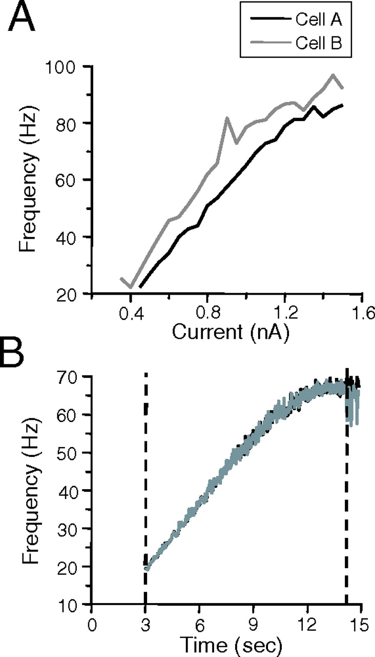
Frequency matching during ramp current injection. A, Individual current versus frequency (f–I) plots for an electrically coupled FS cell pair (cs of 0.31). B, The f–I plots in A were used to construct current ramps that could be simultaneously injected into each cell to drive them at approximately the same intrinsic frequencies over 15 s. The frequency of the two coupled cells in response to the simultaneous ramp current injection is shown. The precise frequency locking in this cell pair results from both the attempt to match intrinsic frequencies and the relatively strong coupling between the cells. Cell A, black lines; cell B, gray lines. Dashed lines indicate the frequency range, with matched frequencies, used for the correlation analysis used in Figure 5.

Analysis of the response of the cell pair to the simultaneous current ramp protocol shown in Figure 4. A, Voltage traces of cell A (black line) and cell B (red line) for a 20 spike window in which the cells fire with a mean frequency of ∼25 Hz. Arrows in C–F correspond to data obtained from this spike window. B, Discrete cross-correlogram obtained from the response shown in A. Note the large central peak near 0 and side bands at the mean interspike interval. C, Running cross-correlogram obtained by concatenating the discrete cross-correlograms of all of the 20 spike windows produced by the ramp, within the dashed lines shown in Figure 4B. The correlation time on the vertical axis corresponds to the correlation time on the horizontal axis of the discrete cross-correlogram in B. The cross-correlation scale on the vertical axis of the discrete cross-correlogram in B is represented by the color scale shown on the right of the running cross-correlogram. The dashed white line and arrow indicates the time at which the discrete cross-correlogram in B was obtained. D, The correlation coefficient CC0 plotted against mean frequency of each 20 spike window. CC0 is taken to be the peak cross-correlation value in a ±5 ms interval centered at 0 (indicated by the solid white lines in C). E, The vector strength (R2) in each 20 spike window during the current ramp plotted against the mean frequency of the window. F, The mean phase in each 20 spike window during the current ramp plotted against the mean frequency of the window. The dashed curves in D and E are p value level curves as determined by the random jitter model. There is a probability p that CC0 and R2 values will be above these curves for uncoupled cell pairs (for details, see text). From bottom to top. p = 0.5, 0.1, 0.05, 0.01, 0.005, and 0.001.
Figure 5A depicts a 20 spike window at an approximate frequency of 25 Hz, which was obtained from the voltage response of the cells to the current ramps illustrated in Figure 4. Note that the heterogeneity of the two FS cells is obvious from the difference in the depths of the action potential afterhyperpolarizations (AHPs). Despite this heterogeneity, the cells were frequency locked and tightly phased locked in synchrony. The discrete cross-correlogram for the 20 spike window in Figure 5A is given in Figure 5B. The tight synchrony of the action potentials is evident by the large correlation coefficient CC0 (0.85) in the discrete cross-correlogram (Fig. 5B), in the running cross-correlogram (Fig. 5C for ±5 ms and dashed line), and in the plot of correlation coefficient versus frequency (Fig. 5D, arrow). It is also evident by the square of the vector strength (R2) close to 1 (Fig. 5E, arrow) and by the mean phase difference (Φ) close to 0 (Fig. 5F, arrow). This example was typical for the relatively strongly coupled pairs (cs > 0.1).
The cross-correlograms computed for all time windows were concatenated to produce a running cross-correlogram (Fig. 5C). The large central peaks in the running cross-correlogram and the corresponding large CC0 values indicate that the cells remained synchronized or almost synchronized over the entire frequency range spanned by the current ramp. The correlation coefficients CC0, the squared vector strengths R2, and the phase differences Φ for each 20 spike window were calculated and plotted against the average frequency of the window (Fig. 5D–F, filled circles). The values of R2 close to 1 also indicate that the cells remained well locked over the entire frequency range. The average phase difference remained very close to 0 in the first half of the ramp but shifted smoothly from 0 to −π/3 at the higher frequencies (50–65 Hz). Note that CC0 remained high in these cases because the phase differences always corresponded to spike-time differences of <5 ms. The apparent loss of tight synchrony at the higher frequencies reflects the larger effect of small spike-time differences with shorter periods and was likely attributable to the heterogeneity of the cells in terms of intrinsic cellular properties or as a result of errors in matching intrinsic frequencies. The conductance-based FS model and G-functions from the experimentally derived PRCs assumed homogeneity in the intrinsic properties of FS cells and did not predict the loss of tight synchrony. However, when heterogeneity in the form of mismatched intrinsic frequencies is introduced in the models, phase shifts in the phase-locked state do indeed occur, e.g., the phase-locked state changes from a synchronous state to an almost synchronous state (Chow, 1998; White et al., 1998; Chow and Kopell, 2000) (see below, Robustness of frequency-locked states increased with coupling coefficient) (supplemental Fig. S6, available at www.jneurosci.org as supplemental material).
The number of spikes used for calculating the cross-correlograms and CC0 values was rather small and could have caused problems in the interpretation of the data. One of the problems is that the time between spikes in the two cells were taken successively rather than chosen randomly from a long spike train and therefore were not independent. Because of the relatively low amount of jitter in the spike trains, high values of CC0 and R2 can occur by chance, and there can be severe bias in the average phase difference. To address this issue, we averaged CC0 and R2 across three trials of the current ramp in each pair. In addition, we used a random jitter model (see Materials and Methods) to compute the statistics of CC0 and R2 values for uncoupled pairs of FS and LTS cells subject to the ramp and step stimulus protocols. Expected values (means) and SDs were computed as a function of firing frequencies. We also computed a measure of significance for the effect of electrical coupling on CC0 and R2 by using p value level curves for CC0 and R2 versus frequency (Figs. 5, 6, dashed lines). For a given measurement of CC0 and R2 in uncoupled cells, there is a probability p that CC0 and R2 would be above the corresponding p value level curve. The p value level curves plotted in Figure 5, D and E, correspond to p = 0.5, 0.1, 0.05, 0.01, 0.005, and 0.001 from bottom to top. As can be seen, the CC0 and R2 are well above chance for this relatively strongly coupled pair of cells.

Population data for pairs of FS and LTS cells obtained with simultaneous current ramps. The average of three trials was used to plot CC0 (top), R2 (middle), and average phase Φ (bottom) against frequency. Each symbol represents a different pair, with the coupling strength (cs) indicated in the legend, and is maintained for all the plots within a column. Open symbols are for pairs with cs < 0.1; filled symbols are for pairs with cs > 0.1. The dashed curves in the plots of CC0 and R2 versus frequency are p value level curves as computed with the random jitter model (black dashed line, p = 0.5; red dashed line, p = 0.005). The data suggests an increase in synchrony with increases in coupling strength but no conclusive dependence of synchrony on frequency.
A complication with the ramp protocol is that the prolonged current injected into cells can have unpredicted effects on the intrinsic currents of the cells. Because this might bias the results, current step protocols were also used. However, the same basic trends seen with the ramp data were also evident in the step data (Fig. 6) (supplemental Fig. S5, available at www.jneurosci.org as supplemental material).
Synchrony and coupling coefficient
The ability of cell pairs to fire within ±5 ms of each other increased with increases in coupling coefficient cs at all frequencies tested. This was true for FS and LTS cells and for pairs with either natural or artificial coupling using dynamic clamp. Running cross-correlograms from cell pairs with relatively strong electrical coupling (cs > 0.1) had fairly large peaks within ±5 ms at all frequencies tested. Conversely, running cross-correlograms from most cell pairs with relatively weak or no coupling (cs < 0.05) had no distinct peaks or small wandering peaks that were inconsistently located from trial to trial. In Figure 6, correlation coefficients CC0, the squared vector strengths R2, and the phase differences Φ that were obtained from current ramps are plotted as functions of frequency for FS and LTS cell pairs with different coupling strengths. Supplemental Figure S5 (available at www.jneurosci.org as supplemental material) shows similar behavior for current steps. In both FS and LTS cell pairs, there is a clear trend for R2 and CC0 values to increase with increases in cs. Note that data points from more weakly coupled cell pairs (cs < 0.05) are not significantly different from the expected values for uncoupled cells that were calculated using the random jitter model (dashed black line). Conversely, data from cell pairs with relatively strong coupling (cs > 0.1) lie above the p = 0.005 level curve (dashed red curve). The phase difference Φ has substantial spread with apparently random variability at low coupling strengths. At higher coupling strengths, Φ tends to be close to 0 and has low systematic variability.
Cross-sections through the CC0 versus frequency plot for the FS cells in Figure 6 are replotted as CC0 versus cs in Figure 7, A and B, for low (∼30 Hz) and high (∼60 Hz) frequencies. This explicitly illustrates the distinct increase in correlation strength with increases in coupling strength. The plot at 30 Hz compares the data obtained from pairs with natural coupling with that obtained by varying the coupling strength in an individual pair with dynamic clamp (filled squares). The slopes of the plots at both 30 and 60 Hz are ∼2.0. The data plotted in Figure 7, A and B, were obtained using a 20 spike window, but the slopes of the plots are similar to that obtained when the correlation was calculated for a larger set of action potential data in which frequency varied over a wide range. This is seen in Figure 7C, in which the correlation coefficient was calculated using a 176 spike window in which the firing frequency varied from 20 to 60 Hz with a mean of 40 Hz.

Synchrony increases with coupling strength. A, FS cell ramp data from Figure 6 at ∼30 Hz are replotted as CC0 versus cs to highlight the relationship between synchrony and coupling strength. The symbols are conserved from Figure 6. Data from an FS cell pair that was dynamically clamped at several coupling strengths are include in the plot (filled squares). B, FS cell ramp data for ∼60 Hz from Figure 6. C, FS cell ramp data calculated using 176 action potentials, with a mean frequency of 40 Hz, averaged over three trials of the ramp protocol for eight pairs with different coupling coefficients. Dashed lines in the top two plots are p value level curves as computed with the random jitter model (p = 0.5; p = 0.005). Solid lines are linear fit to the data points.
Correlation induced by electrical coupling was independent of frequency
The slopes of the linear fits to the CC0 versus frequency data in Figure 6 (supplemental Fig. S5, available at www.jneurosci.org as supplemental material) seem to suggest that the level of synchrony increases with firing frequency. This trend is most apparent in the FS cell data, because they span a greater range of frequencies. However, it is likely that the trend does not result from the interactions of cells through electrical coupling.
Several factors unrelated to coupling contribute to the increase in CC0 with frequency. The two primary factors are as follows: (1) a fixed bin size of 1 ms was used to compute CC0 (independent of frequency), and (2) as frequency is increased, there is a decrease in effective jitter (as measured by the coefficient of variation of ISIs in individual cells) (supplemental Fig. S1, available at www.jneurosci.org as supplemental material). To help separate the effects of electrical coupling from these confounding factors, we compared the CC0 versus frequency data with corresponding expected values for uncoupled cells (as determined by the random jitter model), which serves as the “baseline” or “chance” correlation. Comparison of the linear fits of the data with the chance correlation suggests that the frequency dependence of synchrony is not a significant feature of the data. The slopes of CC0 versus frequency data for both the weakly coupled and the more strongly coupled cells are similar to those predicted for chance correlation.
The independence of synchrony on firing frequency is also evident elsewhere in the cell pair data. The similarity in the slopes of the lines fit to the CC0 versus cs data for FS cells at low and high frequencies (Fig. 7) suggests independence of synchrony on firing frequency. The R2 values, which are a measure of the tightness of phase locking and avoid all data binning issues, show no clear dependence on frequency (Fig. 6) (supplemental Fig. S5, available at www.jneurosci.org as supplemental material).
The experimentally generated G-functions also provided evidence that the increase of CC0 with frequency was not related to electrical coupling. We used our experimentally generated G-functions in conjunction with a method described by Pfeuty et al. (2005) to compute a steady-state correlation coefficient (see Appendix). When calculating the steady-state correlation coefficient, we used two different models for the intrinsic noise of the cells. In the first model, we used intrinsic cellular noise described by the statistics of our jitter measurements from individual cells in which the coefficient of variation of the jitter decreased with frequency (supplemental Fig. 1, available at www.jneurosci.org as supplemental material). In this case, we found a clear increase of correlation coefficient with frequency. In the second model, we used intrinsic cellular noise with a coefficient of variation of the jitter that was independent of frequency and corresponded to the noise level in FS cells firing at 30 Hz. In this case, the correlation coefficients were independent of frequency (supplemental Fig. S7, available at www.jneurosci.org as supplemental material). This suggests that the increase in correlation coefficient with frequency is not attributable to interactions through electrical coupling but rather is a result of an increased chance correlation attributable to the decrease in effective intrinsic noise with increased frequency.
For the more weakly coupled pairs of cells, the average phase difference Φ varies randomly with frequency (Fig. 6) (supplemental Fig. S5, available at www.jneurosci.org as supplemental material). This is attributable to random initial phase differences and subsequent jitter. This conclusion is reinforced by the fact that there is high variability of Φ over all three individual trials and not just in the average as a function of frequency. The Φ values for the more strongly coupled cells are more consistent than those for weakly coupled cells. However, even Φ values for the strongly coupled cells have a tendency to deviate from 0 at high frequencies (Figs. 5F, 6) (supplemental Fig. S5, available at www.jneurosci.org as supplemental material). As mentioned previously, the deviation from synchrony could be attributable to heterogeneity in intrinsic properties of the cells or attributable to mismatched firing frequencies (see next section, Robustness of frequency-locked states increased with coupling coefficient).
Robustness of frequency-locked states increased with coupling coefficient
The theory of weakly coupled oscillators (see Appendix) predicts that, when cells have a sufficiently small difference in intrinsic firing frequencies, cells will phase lock and fire at the same frequency (i.e., frequency lock). The difference in intrinsic frequency will merely lead to a phase shift from the original phase-locked state, e.g., from a synchronous state to an almost synchronous state (supplemental Fig. S6, available at www.jneurosci.org as supplemental material). However, when the difference in intrinsic firing frequencies is increased past a critical value, 1:1 phase locking and frequency locking are lost. The theory predicts that the range of frequencies over which cells frequency lock increases linearly with coupling strength (see Eq. 2 and Appendix).
To explicitly assess the ability of electrical coupling to overcome differences in intrinsic frequencies (i.e., a factor of heterogeneity that can be controlled), we injected a constant current into one cell of a pair while applying a current ramp to the second cell. Thus, the first cell had an approximately constant intrinsic frequency (the holding frequency), whereas the second ramped through a range of intrinsic frequencies. We measured the range of frequencies over which cells fired within ±0.5 Hz of each other and took this to be the range of frequencies over which cells were frequency locked.
Figure 8A shows an example for a relatively strongly coupled FS cell pair (cs of 0.17) in which the holding frequency of the first cell was ∼45 Hz (red trace) and the range of frequency locking (Δf) was ∼5 Hz. Figure 8B shows Δf as a function of the coupling coefficient cs for cell pairs in which one cell was held at ∼45 Hz. The data were derived from four cell pairs with natural coupling (open symbols) and a pair dynamically clamped at four different coupling strengths (filled squares). As theory predicts, Δf increased with increases in cs. A linear fit to the data Δf versus cs gives a slope of 39 Hz. Figure 8C plots the relationship between the coupling strength and the estimated minimum and maximum intrinsic frequency difference for which 1:1 phase and frequency locking occurred, thus showing the boundaries of the frequency-locking region. Figure 8D shows a similar figure for the FS cell pair model, in which the intrinsic frequency of one cell was held constant at 50 Hz. The symbols are the data from direct numerical simulations, and the solid lines are predictions using the theory of weakly coupled oscillators. The increase of the width of the frequency-locking region (Δf) with coupling strength in both model and experiments yields a cusp or triangular shape referred to as an Arnold tongue (Kuznetsov, 1998; Coombes et al., 2001). The skew in the experimental tongue is likely attributable to the ramp protocol and the relatively slow timescale to attain phase locking.

Effects of heterogeneity on phase locking. A, The frequency of one cell in an FS cell pair (cs of 0.17) was increased (black line), whereas the other cell received a constant applied current in an attempt to maintain a fixed intrinsic frequency, i.e., the holding frequency (red line). The solid black line indicates the approximate holding frequency (∼41 Hz). The dashed lines represent the range of frequencies over which the cells fired within ±0.5 Hz of each other. We took this to be the range of frequency locking. The range of frequency locking (Δf) for this pair was ∼5 Hz. Inset, Frequency-locked region on a magnified scale. B, Δf versus coupling coefficient cs for four pairs of cells with natural coupling and for a cell pair that was dynamically clamped at four different coupling strengths (filled squares). The holding frequencies were between 40 and 50 Hz. C, The minimum and maximum frequencies at which pairs were frequency-locked was plotted in relation to the holding frequency for the cell pairs in B. D, The 1:1 phase-locking/frequency-locking region for model FS cells as a function of the difference in the intrinsic frequencies. The holding frequency was 50 Hz. The width of the phase-locking region increases proportionally with coupling strength gcoup. The resulting cusp shape is referred to as an Arnold tongue. (An experimental realization of an Arnold tongue for the real FS cells is shown in C.) All lines in D and F are calculated using the theory of weakly coupled oscillators. The upside-down gray triangles indicate the minimum and maximum frequency differences found from direct numerical simulation of the full FS cell pair model. For coupling coefficients below cs of ∼0.1, there is excellent quantitative agreement between the values from the simulations and the theory of weakly coupled oscillators. Above cs of ∼0.1, small discrepancies begin to appear, particularly at higher frequencies. E, Δf normalized by the coupling strength versus holding frequency of the fixed-frequency cell for five pairs. F, Robustness of the phase-locked states in the model FS cell pair as a function of holding frequency. The black line indicates the maximal difference in frequency for which the stable synchronous phase-locked activity existed; the gray line indicates the maximal frequency difference for which the stable antiphase activity existed. The electrical coupling conductance gcoup was set to 1 nS (cs of 0.1), but the maximal difference in frequency is proportional to gcoup (i.e., cs). When antiphase activity exists, it is much less robust than the synchronous activity.
Figure 8, B and C, shows that, for holding frequencies of ∼45 Hz, the real cell pairs with cs of ∼0.1 remained frequency locked for differences in frequencies less than approximately ±5% (supplemental Fig. S6, available at www.jneurosci.org as supplemental material). Figure 8D shows that, for a holding frequency of 50 Hz, FS model cells with cs of 0.1 remained frequency locked for differences in frequencies below ±8%. Cell pairs modeled using the experimental PRC data in Figure 2, A and B, remained frequency locked (and phase locked) for differences in frequency less than ±6% at a holding frequency of 50 Hz and cs of 0.1 (supplemental Fig. S6, available at www.jneurosci.org as supplemental material). Thus, experimentally measured robustness of phase locking compare well with that found in the FS model and that predicted using the experimentally determined PRCs at ∼40–50 Hz.
Figure 8E plots the size of Δf normalized by the coupling strength as a function of the holding frequency of the second cell for five pairs with different coupling strengths cs. The range of frequency locking (Δf) increases with cs, but there is no clear relationship between this range and the holding frequency (in terms of absolute frequencies range or percentages of the holding frequency). This was confirmed statistically by comparing the means of the data binned between 30–50 and 50–70 Hz (p = 0.5). For the FS cell pair model, Δf for the (almost) synchronous state increased with frequency (Fig. 8F). However, when normalized by the holding frequency Δf/f̄, there was very little dependence on intrinsic frequency. Given a coupling coefficient cs of 0.1, frequency locking in the model persisted for ±7–8% difference in intrinsic frequency. Similar results were found for cell pairs modeled using the experimental PRC data, with values of Δf/f̄ varying from cell pair to cell pair in the range of ±4–8%. Note that, for cs of 0.1, the antiphase state found in the FS cell model at 20 Hz only persisted for differences in intrinsic frequencies less than ∼4%, falling progressively to 0% at ∼30 Hz (Fig. 8F, gray line).
For differences in intrinsic frequencies immediately outside of the frequency-locking region, cells fired at slightly different frequencies, drifting in and out of phase. Farther beyond the frequency-locking region, higher-order phase locking can occur. For example, when the frequency of one cell is approximately twice that of the other, cell pairs can lock in a 2:1 phase-locked state (Ermentrout, 1981) (supplemental Fig. S8, available at www.jneurosci.org as supplemental material).
No evidence for antiphase activity in real interneurons
Our FS cell pair model and other conductance-based models predict that synchronous and antiphase activity can both be stable at sufficiently low firing frequencies (Skinner et al., 1999; Pfeuty et al., 2003; Nomura et al., 2003; Lewis and Rinzel, 2004; Di Garbo et al., 2005; Bem et al., 2005), but this bistability was not evident in our previously described experiments. To fully test the possibility of bistability in real cells, we forced cells into antisynchrony and measured the number of action potentials it took to lose the antisynchronous state. FS cell (n = 5) and LTS cell (n = 2) pairs were injected with 3 s currents steps to bring them to a common firing frequency of 20–50 Hz. After an initial interval of 1 s, during which coupled cells tended to fire in synchrony, cells were paced antisynchronously with a set of 4–8, 2 ms, suprathreshold current pulses.
Three of the FS cell pairs had relatively strong coupling (cs > 0.1) and returned to within a ±5 ms window of synchrony immediately after pacing (within 1–2 action potentials). These pairs remained in synchrony for the remainder of the trial, which consisted of 22.2 ± 7.9 (cs of 0.17), 67.4 ± 1.3 (cs of 0.3), and 34.6 ± 4.6 (cs of 0.31) action potentials (n = 6, 7, and 9 trials, respectively). Similarly, one of the LTS cell pairs had relatively strong coupling (cs of 0.32) and returned to within ±5 ms of synchrony after one action potential, remaining in synchrony for the remainder of the trial (10.0 ± 3.8 action potentials; n = 24 trials). Figure 9A shows the running cross-correlogram for one trial of the antisynchrony protocol for the most strongly coupled FS cell pair. As described above, this pair returned immediately to synchrony after being forced into antisynchrony with eight alternating pulses.

To fully explore the possibility of bistability between synchronous and antisynchronous activity, cells were forced into antisynchrony with eight alternating pulses. A, Running cross-correlogram for one trial of the antisynchrony protocol for a strongly coupled FS cell pair (cs of 0.31). This pair returned immediately to synchrony. B, Running cross-correlogram for one trial of the antisynchrony protocol for a weakly coupled LTS cell pair (cs of 0.04). This pair returned to synchrony more slowly than the strongly coupled pairs.
The weakly coupled (cs of 0.02) FS cell pair stayed in the ±5 ms window around antisynchrony for 9.6 ± 4.3 action potentials (n = 18 trials). It is important to note that even uncoupled cells can remain in the ±5 ms window of antisynchrony (or any other phase difference) for several action potentials attributable to the relatively low jitter of the ISIs. Using a mean ±SD ISI of 23 ± 0.75 ms (as was measured for the cells in this pair), the random jitter model predicted that the cells would leave this window around antisynchrony in 29.2 ± 22.6 action potentials. This suggests the existence of an unstable, and therefore repelling, antisynchronous state. The second LTS cell pair was weakly coupled (cs of 0.04) and returned to within ±5 ms of synchrony much more slowly (12.0 ± 5.5 action potentials) than the strongly coupled pairs, remaining in synchrony for only 5.3 ± 1.7 action potentials (n = 24 trials). This pair remained in antisynchrony after the forcing for 3.3 ± 1.7 action potentials. Figure 9B shows the running cross-correlogram for one trial of the weakly coupled LTS cell pair.
These data strongly suggest that the antiphase state is not stable in electrically coupled pairs of real cortical interneurons.
Decreased AHP size and increased spike width destabilize the antiphase state
The theory of weakly coupled oscillators demonstrates how the shape of the PRCs and the membrane time course of the cells combine to produce phase-locked activity (see Appendix). Here, we examine the influence of the shape of voltage traces and the PRC on the stability of phase-locked states, the antiphase state in particular.
The default experimental G-function computed from the experimentally measured voltage trace and the PRC for a real FS cell firing at 28 Hz is shown as a dashed curve in Figure 10A (same as in Fig. 2B). This G-function has a negative slope at φ = 0, 2π and a positive slope at φ = π, indicating that the synchronous state is stable and the antiphase state is unstable. The dashed curve in Figure 10B is the default model G-function computed from the voltage trace VM(t) and the PRC ZM(t) for the FS cell model firing at 28 Hz. This G-function has a negative slope at φ = 0, 2π and φ = π, indicating that both the synchronous state and the antiphase state are stable.

Shapes of membrane potential trajectories determine stability of the antiphase state. The default G-functions for a real FS cell pair (as in Fig. 2B) and the model FS cell pair at 28 Hz are shown as dashed lines in A and B, respectively. Only synchrony is stable for the real cell pair, and both synchrony and antiphase are stable for the model cell pair. A, When the G-function is computed using the experimental PRC and the model voltage trajectory instead of the experimental voltage trajectory, the antiphase state becomes (weakly) stable (solid curve). B, When the G-function is computed using the model PRC and the experimental voltage trajectory instead of the model voltage trajectory, the antiphase state becomes highly unstable.
To assess whether the shape of the voltage trace or that of the PRC has the predominate effect on the stability of the antiphase state, we computed new G-functions using (1) the experimental PRC and the model voltage trace, and (2) the model PRC and the experimental voltage trace. Figure 10A shows that replacing the voltage trace of the model cell with the experimental voltage trace destabilizes the antiphase state as indicated by the positive slope at φ = π in the new G-function (Fig. 10A, solid curve). Conversely, Figure 10B shows that replacing the experimental voltage trace with that of the model FS cells stabilizes the antiphase state as seen by a slightly negative slope at φ = π in the new G-function (Fig. 10B, solid curve). This implies that the differences between the stability of the antiphase states in the model FS cells and the real FS cells are primarily attributable to the differences in the shapes of the voltage traces and that the differences in the shapes of the PRCs have secondary (more subtle) effects.
Two striking differences between the voltage trace of the real FS cells and that of the model FS cells are as follows: the spike widths, which are considerably thinner in the model cells, and the action potential AHPs, which are substantially larger in the model cells. To examine the influence of these two factors on phase locking, we artificially altered the membrane potential of the real cells while maintaining the default PRC and calculated the corresponding G-functions. Figure 11A shows the default voltage trace (dashed line) and the voltage trace with an added AHP (solid line). Figure 11B compares the corresponding G-functions. The addition of the AHP makes the slope of the G-function at φ = π less positive. That is, the larger AHP has a stabilizing effect on the antiphase state. Note that the added AHP has very little effect on the synchronous state φ = 0, 2π. Figure 11, C and D, shows the default voltage trace (dashed line) with that in which the spike is scaled to be three times thinner (solid line) and compares the corresponding G-functions. The thinner spike results in an overall decrease in the amplitude of the G-function. That is, the decreased spike width destabilizes both the antiphase state and the synchronous state. Figure 11, E and F, shows that combining the increased AHP size and the decreased spike width leads to bistability of the antiphase and the synchronous state, as seen for the model FS cells.

Decreased spike width and increased size of AHP promote antiphase activity. Dashed lines are the default experimental membrane potential V0(t) and G-function at 28 Hz as shown in Figure 2B. The default experimental PRC from Figure 2B is used to compute all of the new G-functions. A, An α-function is added to the default membrane potentials V0(t) to produce a new V0(t) with a larger AHP. B, G-function for V0(t) with the enhanced AHP has a smaller positive slope than the default G-function, indicating that antiphase state is less unstable. C, Spike width of the default membrane potentials V0(t) is scaled down by a factor of 4, producing a new V0(t) with a much thinner spike. D, G-function for V0(t) with a decreased spike width appears to scale down G-function, indicating a reduced stability of both the antiphase and synchronous states. E, V0(t) with both enhanced AHP from A and decreased spike width from C. F, G-function for V0(t) with both enhanced AHP and decreased spike width shows that both the synchronous and antiphase states are now stable.
These results demonstrate that both decreased AHP size and increased spike width destabilize the antiphase state, but AHP size plays a more specific role. These two factors are sufficient to account for the differences in phase locking seen between the real FS cells and the FS cell model. Note also that LTS cells have larger (taller and wider) spikes and smaller AHPs than FS cells, and they do not exhibit stable antisynchrony despite firing at lower frequencies than FS cells. Finally, we should point out that, although we have manipulated the shapes of the PRCs and the membrane time courses of the cells as if they were independent entities, they are in fact intimately related physiologically. In general, changes in intrinsic membrane conductances simultaneously alter both the PRCs and the membrane potential trajectories.
Discussion
Experimental studies have demonstrated the prevalence of electrical coupling between neurons in many vertebrate brain areas (Connors and Long, 2004). These studies have shown that electrical coupling promotes synchrony wherever it is sufficiently strong but have been limited in their analysis of the conditions leading to synchrony. Modeling studies have systematically examined the synchronizing ability of electrical coupling (Chow and Kopell, 2000; Lewis and Rinzel, 2003; Nomura et al., 2003; Pfeuty et al., 2003; Bem et al., 2005; Saraga et al., 2006), but their results have not been verified in real cortical interneuron pairs.
We performed a systematic analysis of phase locking in real pairs of FS and LTS interneurons and in a conductance-based model of an FS cell pair. We used PRCs and the theory of weakly coupled oscillators to make predictions about phase-locking characteristics in cell pairs. Predictions were tested against experiments designed to drive electrically coupled pairs of interneurons through a wide range of firing frequencies. Predictions obtained using experimentally determined PRCs accurately described phase locking in cell pairs. Despite the significant difference in the biophysical properties of FS and LTS cells (Table 1), their phase-locking behavior was remarkably similar. Over the entire frequency range studied, electrical coupling produced only synchrony, which was robust to ∼10% heterogeneity in intrinsic frequencies of cells. Furthermore, the synchronizing ability of electrical coupling and its robustness to heterogeneity was directly dependent on the strength of coupling but not on firing frequency.
Phase–response curves
PRCs measure the sensitivity of cells to external perturbations at different phases in the oscillatory cycle of the cells. In conjunction with the theory of weakly coupled oscillators, PRCs can be used to predict phase-locking dynamics (Kuramoto, 1984; Kopell and Ermentrout, 2002; Lewis and Rinzel, 2003). Experimentally derived PRCs have been obtained for neocortical pyramidal cells (Reyes and Fetz, 1993a,b) and hippocampal neurons (Netoff et al., 2005a). These PRCs have been used to study the influence of chemical synapses on phase-locking behavior (Ermentrout and Kleinfeld 2001; Gutkin et al., 2005; Netoff et al., 2005a). To the best of our knowledge, we provide the first examples of experimentally determined PRCs for neocortical interneurons and the first study that uses experimentally determined PRCs to examine the effects of electrical coupling on phase locking of spiking neurons.
Predictions obtained using PRCs and the theory of weakly coupled oscillators are quantitatively accurate for sufficiently weak coupling (cs of ∼0.1 or less), but the qualitative picture often extends to moderate coupling and realistic network behavior (Netoff et al., 2005b). Because electrical coupling between individual pairs of cortical interneurons is weak, the theory of weakly coupled oscillators is applicable. Indeed, we found that phase-locking results obtained using the theory of weak coupling with experimentally determined PRCs agree with the phase locking of real interneurons.
Synchrony and electrical coupling
In experiments with real cell pairs and in simulations of the FS cell model, electrical coupling was able to synchronize the firing over all frequencies studied (FS, ∼25–80 Hz; LTS, ∼10–30 Hz). The model also exhibited stable antiphase firing at frequencies below ∼30 Hz. Stable antiphase activity has also been found at relatively low frequencies in several other conductance-based models of electrically coupled interneurons (Skinner et al., 1999; Pfeuty et al., 2003; Nomura et al., 2003; Lewis and Rinzel, 2004; Di Garbo et al., 2005; Bem et al., 2005). However, we found no evidence for stable antiphase activity in real cell pairs even when they were forced with antiphase stimuli. It is possible that stable antiphase activity existed in real cell pairs but was too fragile to be observed in the presence of noise and heterogeneity. Previous experiments on pairs of spiking interneurons connected by real (Gibson et al., 2005) and simulated (Merriam et al., 2005; Bem et al., 2005) electrical coupling also failed to reveal antiphase activity.
Evidence for stable antiphase spiking was absent from predictions made with the experimentally derived PRCs and pairs in which electrical coupling was simulated using dynamic clamp, indicating that the discrepancy between experimental and modeling results is not attributable to assumptions of the weak coupling theory or to the fact that electrical coupling was modeled as an ohmic resistance without taking into account dendritic filtering (Alvarez et al., 2002; Lewis and Rinzel, 2004; Saraga and Skinner, 2004; Saraga et al., 2006). It appears that the conductance-based FS model does not adequately capture some fundamental intrinsic properties of real FS cells. Indeed, Pfeuty et al. (2003) showed that small changes in certain intrinsic conductances in models of electrically coupled cells can stabilize antiphase activity (e.g., increasing persistent Na+ conductance). In addition, there is substantial variability in the critical frequencies below which antiphase activity is stable in different models of fast-spiking interneurons (Skinner et al., 1999; Nomura et al., 2003; Pfeuty et al., 2003; Lewis and Rinzel, 2004; Di Garbo et al., 2005). In the study by Di Garbo et al. (2005), stable antiphase activity existed for frequencies up to ∼80 Hz and was quite robust. In the conductance-based model used here, stable antiphase activity found at frequencies of ∼20–30 Hz was fairly fragile to heterogeneities and noise.
Despite their drastically different intrinsic properties, electrically coupled LTS and FS cell pairs both exhibited only robust synchrony. This prompts the question, What properties give these cells the ability to robustly synchronize over a broad range of frequencies and the inability to phase-lock in antiphase? The theory of weakly coupled oscillators provides a way to understand how the shape of the PRCs and the membrane potential trajectory of cells combine to produce specific phase-locking behavior (see Eq. 2). Pfeuty et al. (2003) have demonstrated previously that antiphase activity in electrically coupled cells can be stable if the phase at which the PRC reaches its maximum occurs sufficiently early in the cycle after the action potential. A clear difference in the location of the peak between our model and experimental PRCs is not present. However, we show that differences in the shape of the action potential lead to differences in phase locking between the model and real cells. This demonstrates that, to identify the conductances responsible for promoting synchronization, we need to understand how intrinsic membrane conductances shape both the PRCs and membrane potential trajectory of individual cells (Ermentrout et al., 2001; Acker et al., 2003; Pfeuty et al., 2003; Gutkin et al., 2005). It is important to note that changes in intrinsic membrane conductances alter both the PRC and membrane potential trajectory simultaneously. Pfeuty et al. (2003) showed that certain potassium conductances promote synchrony in a model of electrically coupled cells; we found that both potassium conductances in our FS cell model (gKv1 and gKv3) promote antiphase behavior (supplemental Figs. S9–S11, available at www.jneurosci.org as supplemental material). Thus, more theoretical and experimental work is necessary to understand how ionic conductances determine phase locking.
Functional significance
Electrical coupling between cortical interneurons is primarily restricted to cells of the same type, i.e., between cells with similar electrophysiological properties (but see Simon et al., 2005; Zsiros and Maccaferri, 2005). Our results suggest that electrical coupling can overcome the relatively small differences in intrinsic properties of similar cells, allowing them to fire in synchrony. This supports the hypothesis that FS and LTS networks form two distinct functional units (Gibson et al., 1999, 2005; Beierlein et al., 2003).
The synchronized firing produced by electrical coupling may serve different purposes in the two interneuron networks. FS cells in layer IV of somatosensory cortex receive strong thalamic input and provide feedforward inhibition onto RS cells (Agmon and Connors, 1992; Gibson et al., 1999; Beierlein et al., 2003). Feedforward inhibition exhibits local synchrony (Swadlow et al., 1998), which is thought to sharpen the receptive fields of principal cells (Miller et al., 2001). The dynamics in the FS cell network are complicated by the fact that FS cells are also interconnected by inhibitory synapses (Gibson et al., 1999; Beierlein et al., 2003). Fast inhibitory synapses tend to promote asynchronous activity at frequencies below ∼75 Hz and often lead to bistability of firing phase (Lewis and Rinzel, 2003; Gibson et al., 2005; Merriam et al., 2005; Pfeuty et al., 2005). LTS cells do not receive strong thalamic input, rarely have inhibitory connections to other LTS cells (Gibson et al., 1999; Beierlein et al., 2003) (but see Porter et al., 2001), and have been shown to produce rhythmic inhibition in principal cells (Beierlein et al., 2000; Deans et al., 2001), which can synchronize principal cell firing (Long et al., 2005).
Synchronous population activity in inhibitory networks appears to be essential for the production of a variety of oscillations in the brain, including gamma frequency oscillations (LeBeau et al., 2003; Hasenstaub et al., 2005). This idea is supported by the impairment in gamma frequency oscillations observed in connexin36 knock-out mice (Buhl et al., 2003). Gamma frequency oscillations are thought to be involved in top-down processes such as sensory information processing, attention, and working memory (Engel et al., 2001; Kahana, 2006; Sejnowski and Paulsen, 2006). These processes could be achieved by intrinsic, synchronous oscillations in various cortical areas encoding the relatedness of neural responses, and thus the robust synchronous activity produced by electrically coupled networks of interneurons could be essential for binding related neural responses across cortical areas.
Appendix
Circular statistics: mean phase difference and squared vector strength
Circular statistics (Batschelet, 1981; Drew and Doucet, 1991) were used to describe phase locking between cells. The mean phase difference between the cells [Φ ϵ (−π, π]] was given by
 where
where
 T is the average period of the oscillations, N is the number of spikes in each spike train window, and τk is the time difference between the kth spikes (or the closest corresponding spikes) in the spike trains of the two cells. The measure R2 = X2 + Y2 was used as a measure of the concentration of individual spike-time differences around the mean. R is referred to as the vector strength.
Random jitter model for phase differences between uncoupled cells
To determine baseline values for R2 and CC0, we designed a random walk model to approximate the expected values and the variability of R2 and CC0 for uncoupled cells responding to our experimental stimulus protocols. We refer to this model as the random jitter model. The SDs of the jitter ς for specific mean periods T were obtained from experimentally derived voltage responses of FS and LTS cells to current steps and ramps injected into a single cell (supplemental Fig. S1, available at www.jneurosci.org as supplemental material). These data were fit with quadratic functions to obtain ς(T) for the two cell types and two different stimulus protocols (for fits, see supplemental data, available at www.jneurosci.org as supplemental material). Artificial spike trains were produced using these statistics; firing times of the jth cell were given by
 where rj,k are normally distributed random numbers. If tj,k + 1 < tj,k + trefractory, then tj,k + 1 were recalculated (trefractory = 2 ms). Spike-time differences, CC0, R2, and Φ for the artificial spike trains were calculated as they were for the spike trains from real pairs. A large number (20,000) of realizations of this random jitter model were used to generate approximate probability distributions. These distributions were then used to estimate the means (expected values) and SDs of the distributions of CC0, R2, and Φ for uncoupled cells. In addition, we computed p values for CC0 and R2, i.e., the levels of CC0 and R2 for which there was a probability p that CC0 and R2 would be above these values for uncoupled cells. Thus, the p values were a measure of the significance of the effect of electrical coupling on CC0 or R2.
The random jitter model was also used to estimate the cumulative probability distribution for the time (in number of spikes) that an uncoupled cell pair would remain within ±1 ms of a fixed phase difference. Cumulative probability distributions were computed for various mean ± SD ISIs using 20,000 realizations. These distributions provided the approximate probability that uncoupled cells would appear phase locked (within ±1 ms) for a given number of spikes purely by chance.
The theory of weakly coupled oscillators: derivation of the G-function
For weak coupling and weak heterogeneity, the theory of weakly coupled oscillators (Kuramoto, 1984; Hansel et al., 1995; Kopell and Ermentrout, 2002; Lewis and Rinzel, 2003) derives an equation governing the phase difference between the coupled cells φ. A brief derivation of this equation is provided below. In this derivation, the cells are assumed to have identical intrinsic properties, and heterogeneity is assumed to arise only from small difference in their applied current.
Assume that two cells are weakly coupled (gcoup is small) and that the cells are driven by applied currents Īapplied + ΔI/2 and Īapplied − ΔI/2, where ΔI is small (the cells are weakly heterogeneous). Take V0(t) to be the oscillatory membrane potential of the uncoupled cells when they receive the applied current Īapplied and Z(t) to be the corresponding PRC. Because the heterogeneity and coupling between cells are weak, the periods of the oscillations of coupled cells are approximately equal to the period of the cell receiving the average applied current, T. Furthermore, the membrane potentials of the cells Vj(t) are approximately equal to V0(t) with the exception that they will have phase shifts
 The electrical coupling current flowing from cell k to cell j is approximately
 Using the PRC and its definition (Eq. 1), the phase shift in cell j attributable to the coupling current from cell k and the heterogeneity in applied current over a brief time Δt is
 Taking the limit of continuous time (Δt→0),
 As a result of the weak heterogeneity and the weak coupling (i.e., the small ΔI and small coupling current), the change in phase occurs on a much slower timescale than the period of the oscillation. Therefore, we can average the right side of the above equation over a period of the oscillation
 or
or
 Defining the phase difference between cells as
 or
or
 which is Equation 2 in Materials and Methods.
The function H, which describes the interaction between the phases of the cell pair, is often referred to as the phase coupling function or the interaction function. Q is the average of the PRC over the period T. We refer to the function G as the cell pair coupling function or the G-function.
We should note that PRCs for the model were not computed using the method described for the in vitro cells (see Materials and Methods). The PRC is the normalized T-periodic solution of the adjoint equation for the isolated FS cell model linearized about the T-periodic limit cycle V0(t) (Kuramoto, 1984; Ermentrout and Kopell, 1991). Solutions to the adjoint equations were computed as described by Williams and Bowtell (1997), using programs written in Matlab (MathWorks, Natick, MA) (Euler method, time step size of 0.001 ms). Example PRCs for frequencies of 30 and 60 Hz were checked against adjoint solutions computed using the software package XPPAUT (Ermentrout, 2002) at these frequencies. The theory of weakly coupled oscillators (Eq. 2) provides a linear relationship between half-width of the frequency-locking region (1:1 phase-locking region) and the coupling strength: ΔI = (Gmax/Q)gcoup, where Gmax is the maximum of the G-function. The ratio ΔI/gcoup= Gmax/Q is the magnitude of the inverse of slopes of the boundaries of the Arnold tongue in Figure 8 and provides a measure of the robustness of the phase-locked states at a particular frequency. Note that phase shifts in the phase-locked states occur as ΔI, and thus the difference in intrinsic frequency is changed.
Pfeuty et al. method to predict the steady-state correlation coefficient
The predicted steady-state cross-correlogram ρ(ψ) using the theory of weakly coupled oscillators (Pfeuty et al., 2005) is
 where G is the predetermined G-function, ςT is the SD of the effective noise in terms of phase. For details, see Pfeuty et al. (2005). In our calculations, we used experimentally determined G-functions, and we set (1) ςT to be equal to the appropriately scaled coefficient of variance of the jitter data in supplemental Figure S1 (available at www.jneurosci.org as supplemental material), or (2) ςT to be a fixed value of 5.5%, which corresponds to the noise level in FS cells firing at 30 Hz. The coefficient of variance of our jitter data for FS and LTS cells decreased with frequency. This resulted from a decreased sensitivity of the cells when they were close to threshold and is reflected by the decreased size of the positive lobe of the PRCs (Fig. 2) (supplemental Figs. S2–S4, available at www.jneurosci.org as supplemental material). We used electrical coupling conductances of 1 and 2 nS. The value ρ(0) is a measure of synchrony and is approximately proportional to the correlation coefficient used throughout this paper, CC0.
Footnotes
-
This work was supported by National Institutes of Health Grants NS25983 and NS050434, the Epilepsy Foundation through the support of the American Epilepsy Society, and the Milken Family Foundation. T.J.L. was supported by National Institute of Mental Health Postdoctoral Fellowship MH12873 and National Science Foundation Grant DMS-0518022. We thank Dr. Z. Josh Huang for supplying us with the G42/C57BL6 mice, C. Dorval and J. A. White for help with the real-time Linux dynamic clamp, H. Abarbanel for the analog circuit dynamic clamp, Jay Gibson for writing LabView software, and Saundy Patrick for her critical technical assistance.
- Correspondence should be addressed to Jaime G. Mancilla at his present address: Department of Otolaryngology/Head and Neck Surgery, 1115 Bioinformatics Building, 130 Mason Farm Road, Campus Box 7070, University of North Carolina, Chapel Hill, NC 27599-7070. mancilla{at}email.unc.edu


